Mastering CTCF ChIP-seq: A Complete Workflow Guide for Chromatin Researchers (2024)
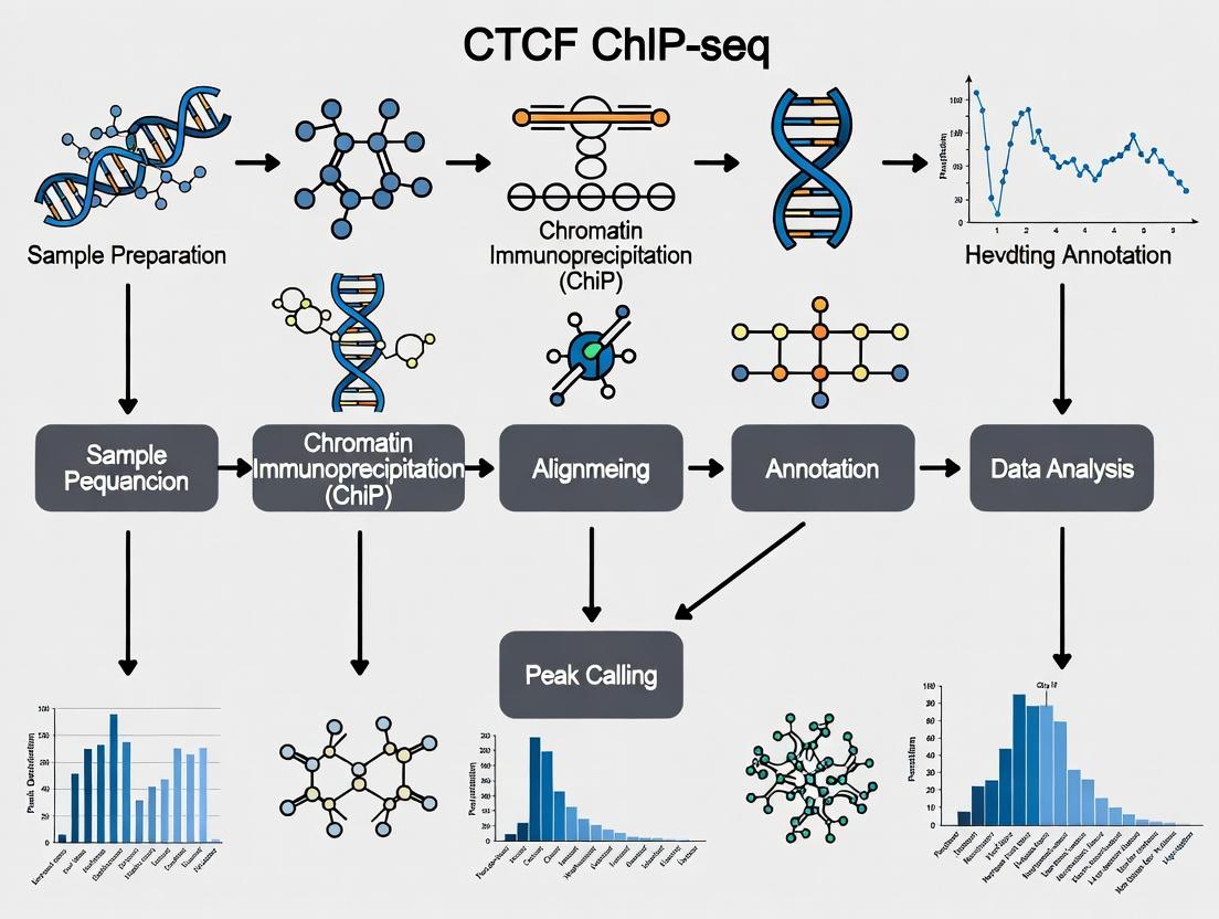
This comprehensive guide provides researchers, scientists, and drug development professionals with a complete, up-to-date workflow for analyzing CTCF ChIP-seq data.
Mastering CTCF ChIP-seq: A Complete Workflow Guide for Chromatin Researchers (2024)
Abstract
This comprehensive guide provides researchers, scientists, and drug development professionals with a complete, up-to-date workflow for analyzing CTCF ChIP-seq data. We begin by establishing the foundational role of CTCF as the 'master weaver' of the genome in 3D chromatin architecture and gene regulation. The methodological core presents a detailed, step-by-step pipeline from raw FASTQ files to high-confidence peak calling and annotation, featuring modern tools and best practices. We address common pitfalls, quality control failures, and optimization strategies for challenging samples. Finally, we explore rigorous validation techniques and comparative analyses against other epigenetic datasets (e.g., Hi-C, ATAC-seq) to derive biological meaning. This article equips you to reliably map insulator sites and topological domain boundaries to advance research in genomics, disease mechanisms, and therapeutic discovery.
CTCF 101: Understanding the Genome's Architect Before You Sequence
Why CTCF? Defining Its Crucial Role as an Insulator Protein and 3D Genome Organizer
Application Notes: CTCF in 3D Genome Architecture and Disease
CTCF (CCCTC-binding factor) is a master architectural protein fundamental to the spatial organization of chromatin. Its primary roles are as an insulator, preventing inappropriate enhancer-promoter interactions, and as a key driver in the formation of topologically associating domains (TADs) and loops, which compartmentalize genome function. In the context of a thesis on CTCF ChIP-seq data analysis, understanding these biological roles is critical for interpreting binding patterns, variant effects, and differential occupancy studies.
Table 1: Quantitative Metrics of CTCF Binding and 3D Genome Organization
| Metric | Typical Range / Value | Experimental Method | Relevance to Analysis Workflow |
|---|---|---|---|
| Genome-wide binding sites (human/mouse) | ~50,000 - 100,000 | ChIP-seq, ChIP-exo | Defines peak calling sensitivity thresholds. |
| Consensus motif occurrence | > 1 million | Sequence analysis | Highlights specificity of in vivo binding vs. motif prediction. |
| Cohesion colocalization at loops | ~60-80% of loops | ChIA-PET, Hi-C | Informs integrative analysis for loop calling. |
| TAD boundaries with CTCF | ~70-90% | Hi-C | Validates TAD boundary calls from chromatin contact maps. |
| Allelic imbalance in binding | Variable (e.g., 10-40% fold-change) | Allele-specific ChIP-seq | Key for analyzing SNPs or mutations affecting binding. |
Table 2: Disease-Associated Genetic Variants in CTCF Sites
| Disease Context | Variant Type | Proposed Consequence | Analysis Challenge |
|---|---|---|---|
| Cancer (multiple types) | Somatic mutations in CTCF motifs | Disrupted insulation, oncogene activation | Distinguishing driver from passenger non-coding variants. |
| Neurodevelopmental disorders | De novo mutations in CTCF or its sites | Altered neuronal gene expression | Linking subtle binding changes to gene dysregulation. |
| Autoimmunity | SNPs in CTCF-bound enhancers | Immune cell dysregulation | Cell-type-specific interpretation of ChIP-seq signals. |
Detailed Protocols
Protocol 1: Standardized CTCF ChIP-seq Wet-Lab Workflow
Objective: To generate high-quality, reproducible chromatin immunoprecipitation sequencing libraries for CTCF.
Key Research Reagent Solutions:
| Reagent / Material | Function | Critical Notes |
|---|---|---|
| Crosslinking Agent (Formaldehyde) | Fixes protein-DNA interactions. | Optimization of fixation time (e.g., 10 min) is crucial to balance signal and background. |
| Anti-CTCF Antibody | Specific immunoprecipitation of CTCF-DNA complexes. | Validated for ChIP-seq (e.g., Millipore 07-729, Diagenode C15410210). |
| Protein A/G Magnetic Beads | Capture antibody-bound complexes. | Bead blocking reduces non-specific background. |
| Chromatin Shearing Apparatus (Sonication) | Fragment chromatin to 200-500 bp. | Must be optimized per cell type; over-sonication damages epitopes. |
| DNA Clean-up Beads (SPRI) | Size selection and purification of libraries. | Maintains fragment size distribution crucial for peak resolution. |
| High-Fidelity PCR Mix & Unique Dual Indexes | Amplify and barcode libraries for multiplexing. | Minimize PCR cycles (≤15) to avoid duplicates and biases. |
Steps:
- Cell Fixation & Harvesting: Crosslink 1-5 million cells with 1% formaldehyde for 10 min at RT. Quench with glycine.
- Cell Lysis & Chromatin Shearing: Lyse cells in SDS buffer. Sonicate chromatin to an average size of 300 bp. Verify fragmentation via gel electrophoresis.
- Immunoprecipitation: Clarify lysate. Incubate supernatant with 1-5 µg of anti-CTCF antibody overnight at 4°C. Add beads for 2 hours. Wash sequentially with Low Salt, High Salt, LiCl, and TE buffers.
- Elution & Decrosslinking: Elute complexes in ChIP elution buffer (1% SDS, 0.1M NaHCO3). Add NaCl and reverse crosslinks at 65°C overnight.
- DNA Purification: Treat with RNase A and Proteinase K. Purify DNA using SPRI beads.
- Library Preparation & Sequencing: Use a dedicated library prep kit (e.g., NEB Next Ultra II) for end-repair, dA-tailing, adapter ligation, and indexed PCR. Sequence on an Illumina platform to a depth of 20-40 million non-duplicate reads.
Protocol 2: In Silico CTCF ChIP-seq Peak and Motif Analysis
Objective: To process raw sequencing data, call peaks, and analyze CTCF motif orientation. Thesis Context: This is the core computational workflow.
Key Research Reagent Solutions (Bioinformatics):
| Tool / Software | Function | Critical Notes |
|---|---|---|
| FastQC/MultiQC | Quality control of raw FASTQ files. | Identifies adapter contamination or quality drops. |
| Trim Galore!/Cutadapt | Adapter trimming and quality filtering. | Preserves read length for accurate alignment. |
| Bowtie2/BWA | Align reads to reference genome. | Use sensitive settings for short ChIP-seq reads. |
| MACS2 | Call significant peaks from aligned reads. | Use --broad flag is not recommended; CTCF peaks are sharp. |
| MEME Suite/HOMER | De novo and known motif discovery. | HOMER's findMotifsGenome.pl is optimized for ChIP-seq. |
| Bedtools | Intersect peaks with genomic features. | Essential for comparing replicates or conditions. |
Steps:
- Quality Control & Alignment: Run FastQC. Trim adapters. Align reads to reference genome (e.g., hg38) using Bowtie2. Filter for uniquely mapped, proper pairs.
- Peak Calling: Call peaks using MACS2 (
macs2 callpeak -t treatment.bam -c control.bam -f BAMPE -g hs -n CTCF --keep-dup all). - Motif Analysis: Extract sequences from peak summits (±50 bp). Use HOMER (
findMotifsGenome.pl) to identify the canonical CTCF motif and its orientation. - Orientation Analysis: Classify peaks based on motif directionality. This is critical for predicting loop anchor compatibility (convergent orientation preferred).
Visualizations
Title: CTCF ChIP-seq Wet-Lab Experimental Workflow
Title: CTCF ChIP-seq Computational Analysis Pipeline
Title: CTCF-Mediated Insulation and Loop Formation Mechanism
This Application Note is framed within a broader thesis research project focused on developing an optimized, end-to-end computational workflow for the analysis of CTCF ChIP-seq data. The central thesis posits that a standardized analytical pipeline, integrating peak calling, motif analysis, loop annotation, and variant interpretation, is critical for reproducibly translating raw sequencing data into biological insights regarding genome architecture and disease mechanisms.
Table 1: Core Biological Questions Answered by CTCF ChIP-seq Analysis
| Biological Question | Primary CTCF ChIP-seq Readout | Typical Quantitative Findings (Based on Current Literature) | Implication for Genome Biology |
|---|---|---|---|
| 1. Where does CTCF bind? | Genome-wide occupancy peaks. | ~30,000 - 80,000 peaks identified per mammalian cell type; ~15-40% are cell-type specific. | Maps insulator protein locations, candidate regulatory elements. |
| 2. What sequences underlie CTCF binding? | De novo motif discovery within peaks. | >90% of peaks contain the core 20-bp motif; motif orientation is functionally relevant. | Identifies canonical and variant motifs; informs binding specificity. |
| 3. How is 3D genome architecture organized? | Co-localization with TAD boundaries and loop anchors. | ~60-70% of TAD boundaries are bound by CTCF; convergent motif orientation is enriched at loop anchors. | Defines architectural role in insulating domains and facilitating enhancer-promoter loops. |
| 4. How do genetic variants alter CTCF function? | Variant overlap with peaks/motifs and associated epigenetic changes. | Disease-associated SNPs from GWAS are enriched in CTCF binding sites (Odds Ratio often 2-5). | Provides mechanism for non-coding variants in disease (e.g., cancer, autoimmunity). |
| 5. How does CTCF contribute to disease states? | Differential binding analysis (e.g., mutant vs. wild-type, diseased vs. healthy). | Hundreds to thousands of sites show loss/gain of binding in cancer cells (e.g., with CTCF mutation or polycomb dysregulation). | Reveals oncogenic disruption of chromatin topology and dysregulated gene programs. |
Detailed Protocols
Protocol 1: Standard CTCF ChIP-seq Wet-Lab Procedure
Adapted from the Van Nostrand Lab Protocol (Current as of 2023).
A. Cell Crosslinking & Lysis
- Crosslink cells in 1% formaldehyde for 10 min at RT. Quench with 125 mM glycine.
- Pellet cells, wash with cold PBS. Resuspend in Lysis Buffer I (50 mM HEPES-KOH pH 7.5, 140 mM NaCl, 1 mM EDTA, 10% Glycerol, 0.5% NP-40, 0.25% Triton X-100) for 10 min on ice.
- Pellet nuclei. Resuspend in Lysis Buffer II (10 mM Tris-HCl pH 8.0, 200 mM NaCl, 1 mM EDTA, 0.5 mM EGTA) for 10 min on ice.
- Pellet nuclei. Resuspend in Shearing Buffer (0.1% SDS, 1 mM EDTA, 10 mM Tris-HCl pH 8.0). Proceed to sonication.
B. Chromatin Shearing & Immunoprecipitation
- Sonicate chromatin to an average fragment size of 200-500 bp. Clarify by centrifugation.
- Dilute sonicated chromatin 1:10 in ChIP Dilution Buffer (0.01% SDS, 1.1% Triton X-100, 1.2 mM EDTA, 16.7 mM Tris-HCl pH 8.0, 167 mM NaCl).
- Pre-clear with Protein A/G beads for 1-2 hours.
- Incubate supernatant with 2-5 µg of anti-CTCF antibody (e.g., Millipore 07-729) overnight at 4°C.
- Add pre-blocked Protein A/G beads and incubate for 2 hours.
- Wash beads sequentially:
- Wash Buffer I (0.1% SDS, 1% Triton X-100, 2 mM EDTA, 20 mM Tris-HCl pH 8.0, 150 mM NaCl)
- Wash Buffer II (0.1% SDS, 1% Triton X-100, 2 mM EDTA, 20 mM Tris-HCl pH 8.0, 500 mM NaCl)
- Wash Buffer III (0.25 M LiCl, 1% NP-40, 1% deoxycholate, 1 mM EDTA, 10 mM Tris-HCl pH 8.0)
- TE Buffer (10 mM Tris-HCl pH 8.0, 1 mM EDTA)
- Elute chromatin in Elution Buffer (1% SDS, 100 mM NaHCO3). Reverse crosslinks at 65°C overnight.
C. DNA Purification & Library Prep
- Treat with RNase A and Proteinase K.
- Purify DNA using phenol-chloroform extraction or SPRI beads.
- Prepare sequencing library using a commercially available kit (e.g., NEB Next Ultra II DNA Library Prep). Include size selection for 200-600 bp fragments.
- Validate library quality (Bioanalyzer) and sequence on an Illumina platform (≥ 20 million reads for mammalian genomes).
Protocol 2: Computational Workflow for Identifying TAD Boundaries & Loops
Core pipeline from the thesis research framework.
- Raw Data Processing:
- Use
fastporTrimmomaticfor adapter trimming and quality control. - Align reads to reference genome (e.g., hg38) using
Bowtie2orBWA. - Remove duplicates with
Picard Toolsorsamtools.
- Use
- Peak Calling & Quality Assessment:
- Call peaks using
MACS2(callpeak -B --SPMR -g hs --keep-dup all). Input DNA is essential. - Assess signal enrichment with
phantompeakqualtools(NSC > 1.05, RSC > 0.8).
- Call peaks using
- Motif Analysis & Orientation:
- Extract sequences from peak summits (±50 bp) using
bedtools getfasta. - Perform de novo motif discovery with
MEME-ChIPand scan for known motifs withHOMER(findMotifsGenome.pl). - Annotate motif directionality relative to the reference genome.
- Extract sequences from peak summits (±50 bp) using
- Architectural Feature Annotation:
- TAD Boundary Calling: Use Hi-C data (from same/similar cell type) with
Arrowhead(Juicer Tools) orInsulationScore(cooltools) to define TADs. Overlap CTCF peaks with boundaries. - Loop Anchor Identification: Use Hi-C data with
HiCCUPS(Juicer Tools) to call loops. Overlap loop anchors with CTCF peaks containing convergent motifs.
- TAD Boundary Calling: Use Hi-C data (from same/similar cell type) with
- Variant Intersection Analysis:
- Overlap peak coordinates with genomic variant files (e.g., GWAS SNPs, cancer mutations from COSMIC) using
bedtools intersect. - For variants within motifs, use
TOMTOMto assess impact on motif score (e.g., withFIMO).
- Overlap peak coordinates with genomic variant files (e.g., GWAS SNPs, cancer mutations from COSMIC) using
Visualizations
Diagram 1: CTCF ChIP-seq Analysis Workflow & Biological Questions
Diagram 2: CTCF, Cohesin, and TAD Boundary Formation
The Scientist's Toolkit: Research Reagent Solutions
Table 2: Essential Reagents & Tools for CTCF ChIP-seq Studies
| Item Name/Code | Supplier Examples | Function in CTCF ChIP-seq | Critical Notes |
|---|---|---|---|
| Anti-CTCF Antibody | Millipore (07-729), Cell Signaling (3418S), Abcam (ab188408) | Immunoprecipitation of CTCF-DNA complexes. | Validate for ChIP-grade specificity; Millipore 07-729 is a widely used benchmark. |
| Protein A/G Magnetic Beads | Thermo Fisher, Diagenode, Millipore | Capture antibody-bound chromatin. | Offer easier washing than agarose beads; reduce background. |
| Micrococcal Nuclease (MNase) | NEB, Worthington | Alternative to sonication for chromatin shearing; can give nucleosome-resolution peaks. | Yields different fragment profiles than sonication; optimal for some protocols. |
| NEB Next Ultra II DNA Library Prep Kit | New England Biolabs | Prepares sequencing libraries from low-input ChIP DNA. | Highly efficient for low-yield ChIP samples; includes size selection. |
| SPRIselect Beads | Beckman Coulter | Size selection and clean-up of DNA after ChIP and library prep. | Critical for removing adapter dimers and selecting optimal fragment size. |
| Cell Line/Tissue with Hi-C Data | ENCODE, 4DN Portal | Matching Hi-C data for architectural analysis (TADs/loops). | Essential for correlating CTCF binding with 3D genome structure. |
| MEME-ChIP Suite | meme-suite.org | De novo motif discovery and enrichment analysis. | Standard for identifying the CTCF motif and potential co-occurring motifs. |
| MACS2 Software | GitHub: macs3-project/MACS | Peak calling from aligned ChIP-seq reads. | Industry standard; use with broad peak mode for some factors, but not typically for CTCF. |
| bedtools Suite | GitHub: arq5x/bedtools2 | Genomic interval arithmetic (intersection, coverage, etc.). | Fundamental for comparing peaks with genes, variants, and other genomic features. |
| Juicer Tools / cooltools | GitHub: aidenlab/juicer; open2c/cooltools | Processing Hi-C data to call TADs and loops for integration. | Required to move from 1D binding maps to 3D architectural insights. |
Within the broader thesis on a CTCF ChIP-seq data analysis workflow, rigorous experimental design and pre-analysis considerations are paramount for generating biologically valid and statistically robust data. This document details the essential protocols and application notes for planning a CTCF ChIP-seq experiment, with a focus on control selection, replicate strategy, and quality assessment to ensure downstream computational analysis yields meaningful insights into chromatin architecture and gene regulation.
CTCF (CCCTC-binding factor) is a critical architectural protein involved in insulator function, enhancer-promoter interactions, and 3D genome organization. ChIP-seq is the primary method for mapping its genome-wide binding sites. The accuracy of subsequent bioinformatic analysis is wholly dependent on the quality of the raw data, which is governed by pre-analytical experimental decisions.
Core Experimental Design Considerations
Biological vs. Technical Replicates
To ensure findings are generalizable and statistically sound, a clear replicate strategy is non-negotiable.
Table 1: Replicate Strategy for CTCF ChIP-seq
| Replicate Type | Definition | Primary Purpose | Minimum Recommended Number | Rationale for CTCF |
|---|---|---|---|---|
| Biological Replicate | Samples derived from distinct biological sources (e.g., different cell cultures, different mice). | Account for biological variation. | 3 (2 absolute minimum) | CTCF binding can vary with genetic background, cell cycle, and subtle environmental changes. |
| Technical Replicate | Multiple library preparations or sequencings from the same chromatin extract. | Account for technical noise from library prep and sequencing. | Usually 1, if sequencing depth is pooled. | High-cost experiment; library prep variability is often assessed via quality metrics (e.g., PCR bottleneck coefficient). |
Control Experiments: Input, IgG, and Beyond
Appropriate controls are essential for accurate peak calling and background subtraction.
Table 2: Control Experiments in CTCF ChIP-seq
| Control Type | Description | Protocol Source | Primary Use in Analysis | Critical Notes |
|---|---|---|---|---|
| Input (Reference) | Chromatin taken prior to immunoprecipitation, fragmented, and processed alongside ChIP samples. | See Protocol 3.2. | Accounts for sequencing bias due to chromatin accessibility, DNA fragmentation, and GC content. The gold standard. | Must use the same cell type and cross-linking conditions. Should be sequenced deeper than individual ChIP samples (e.g., 2x coverage). |
| IgG (Negative) | Immunoprecipitation with a non-specific immunoglobulin (same host species as ChIP antibody). | See Protocol 3.3. | Identifies non-specific antibody binding and background noise. Useful for assessing signal-to-noise. | Often less effective than Input for peak calling with modern algorithms. Can be used in conjunction with Input. |
| Positive Control Locus | A genomic region with a well-characterized, strong CTCF binding site (e.g., MYC insulator, H19/Igf2 ICR). | Validated via literature and qPCR. | Quality control (QC) to confirm successful ChIP experiment prior to sequencing. | Failed positive control indicates a problem with the ChIP wet-lab protocol. |
Detailed Protocols
Protocol 3.1: Cell Harvesting and Cross-linking for CTCF
Objective: Fix protein-DNA interactions in situ. Reagents: Cell culture, 37% Formaldehyde (Methanol-free), 2.5M Glycine, PBS. Steps:
- For adherent cells, add 1% final concentration formaldehyde directly to culture medium. Rotate 10 minutes at room temperature (RT).
- Quench cross-linking by adding glycine to a final concentration of 0.125M. Incubate 5 minutes at RT.
- Aspirate medium, wash cells twice with cold PBS.
- Scrape cells, pellet at 500 x g for 5 min at 4°C. Flash-freeze pellet in liquid N₂ or proceed to sonication.
Protocol 3.2: Input DNA Preparation
Objective: Generate the reference control library. Reagents: Cell pellet, Lysis Buffer, RNase A, Proteinase K, Phenol-Chloroform. Steps:
- Take 10% of the cross-linked cell suspension before adding the ChIP antibody.
- Reverse cross-links: Add RNase A (30 min, 37°C), then Proteinase K (2 hrs, 65°C).
- Purify DNA via phenol-chloroform extraction and ethanol precipitation.
- Resuspend DNA. This "Input DNA" is used for subsequent library preparation alongside ChIP DNA.
Protocol 3.3: Non-Specific IgG Control ChIP
Objective: Perform immunoprecipitation with a control antibody. Reagents: Pre-cleared chromatin, Normal Rabbit/IgG (species-matched to CTCF antibody), Protein A/G Magnetic Beads, all ChIP buffers. Steps:
- Follow the same ChIP protocol as for the target antibody (CTCF).
- Substitute the specific CTCF antibody with an equivalent mass of non-specific IgG (e.g., 1-5 µg).
- Process in parallel through all wash steps, elution, and reverse cross-linking.
- Purify DNA. The yield should be significantly lower than the specific ChIP.
The Scientist's Toolkit
Table 3: Essential Research Reagent Solutions for CTCF ChIP-seq
| Item | Function / Purpose | Example / Note |
|---|---|---|
| Methanol-free Formaldehyde | Cross-links proteins to DNA. | Essential for capturing transient or weak CTCF-DNA interactions. Methanol can inhibit cross-linking. |
| CTCF-specific Antibody | Immunoprecipitates the target protein-DNA complex. | Critical for success. Use validated ChIP-seq grade antibodies (e.g., Millipore 07-729, Diagenode C15410210). |
| Protein A/G Magnetic Beads | Efficient capture of antibody-protein-DNA complexes. | Facilitates quick wash steps and reduces background compared to agarose beads. |
| Sonication Device | Fragments cross-linked chromatin to 200-500 bp. | Covaris focused-ultrasonicator is preferred for consistent shearing. Bioruptor is a common alternative. |
| DNA Size Selection Beads | Clean up DNA after elution and select optimal fragment size for library prep. | SPRI/AMPure XP beads are standard. |
| High-Fidelity PCR Master Mix | Amplifies ChIP and Input libraries for sequencing. | Use low-cycle PCR (8-15 cycles) to minimize duplicates and bias. |
| DNA High Sensitivity Assay | Quantifies low-concentration DNA post-ChIP and library prep. | Qubit dsDNA HS Assay or TapeStation. |
Visualization of Workflows and Concepts
Diagram Title: CTCF ChIP-seq Experimental Workflow
Diagram Title: Control Selection Logic for Peak Calling
This document provides detailed application notes and protocols for mining public data repositories for CTCF ChIP-seq datasets. This work is part of a broader thesis on establishing a robust, reproducible workflow for the acquisition, processing, and analysis of CTCF binding data, a critical factor in chromatin architecture and gene regulation. The notes are designed for researchers, scientists, and drug development professionals seeking to leverage existing public data for hypothesis generation and validation.
Table 1: Comparison of Major Public Data Repositories for CTCF ChIP-seq
| Repository | Primary Focus | Key Features for CTCF Data | Estimated CTCF Datasets (as of 2024) | Data Format & Metadata | Access Method |
|---|---|---|---|---|---|
| ENCODE | Comprehensive functional genomics | Highly standardized, uniformly processed, extensive metadata (cell type, antibody, replicates). | ~1,200 (Human & Mouse) | Processed peaks (BED), signal tracks (bigWig), raw data (FASTQ). | Portal website, REST API, direct download. |
| GEO (NCBI) | Archive for high-throughput data | Vast volume, diverse experimental conditions, includes published and unpublished data. | ~4,000 Series | Raw (FASTQ/SRA), processed files vary widely by submitter. | Web browser, SRA-Toolkit, GEOquery (R). |
| Cistrome DB | Curated chromatin profiles | Quality-filtered, uniformly processed (using Cistrome pipeline), integrated analysis tools. | ~2,800 (Human & Mouse) | Consistent peak calls (BED), signal tracks, quality metrics. | Gateway website, Data Browser. |
Protocols for Dataset Mining
Protocol 1: Systematic Retrieval of CTCF Data from ENCODE
Objective: To identify and download uniformly processed CTCF ChIP-seq datasets for specific cell lines or tissues.
- Access the ENCODE Portal: Navigate to
www.encodeproject.org. - Apply Filters: Use the search/filter interface.
- Target of assay:
CTCF(from "Target gene" list). - Assay title:
ChIP-seq. - Organism:
Homo sapiensorMus musculus. - Biosample term: e.g.,
K562,HepG2,heart. - File format: Select
bed narrowPeak(for peak calls) andbigWig(for signal). - Output type:
peaksandsignal of unique reads. - Assembly:
GRCh38ormm10.
- Target of assay:
- Quality Check: Prioritize datasets with:
- Status:
released. - Audits: No
ERRORorWARNINGaudits. - Biological replicates: At least two.
- Files: Both replicate and optimal IDR thresholded peak files available.
- Status:
- Bulk Download: Select desired files, click "Download", and use the generated
tsvfile withcurlorwgetfor command-line retrieval.
Protocol 2: Mining GEO for CTCF Studies and Raw Data
Objective: To find both raw sequencing data and associated metadata for CTCF ChIP-seq experiments under specific biological conditions (e.g., disease, treatment).
- GEO Text Search:
- Go to
www.ncbi.nlm.nih.gov/geo/. - Use the advanced search:
"CTCF"[All Fields] AND "ChIP-seq"[All Fields] AND "Homo sapiens"[Organism]. - Filter by
Seriesto get entire studies.
- Go to
- Refine Results: Scan titles and abstracts. Use the
GEO2Ranalysis link to preview sample metadata table (GSMentries) for cell type, antibody, and treatment details. - Access Raw Data (SRA):
- From a
GSEpage, link to theSRA Run Selector. - Identify the
SRRaccessions for CTCF samples.
- From a
Download using SRA-Toolkit:
Programmatic Access with GEOquery (R/Bioconductor): For metadata and processed data.
Protocol 3: Leveraging Cistrome DB for Quality-Filtered Data
Objective: To quickly obtain pre-processed, quality-controlled CTCF datasets and their quality metrics.
- Access the Data Browser: Navigate to
cistrome.org/db/#/browse. - Set Browse Criteria:
- Factor: Search and select
CTCF. - Species:
HumanorMouse. - Cell/Tissue: Type to filter.
- Quality: Set a threshold (e.g.,
>= 1or>= 2). The Cistrome Quality Score (CQS) integrates sequencing and peak calling metrics.
- Factor: Search and select
- Evaluate and Select: Browse results sorted by CQS. Click on a sample to view detailed metrics (SPOT score, FRiP, peak number) and sample info.
- Download: Click the download icon for a sample to retrieve peak files (BED) and signal tracks (bigWig) processed through a uniform pipeline.
Diagrams
DOT Code for Diagram 1: CTCF Dataset Mining Workflow Decision Tree
Title: Decision Tree for Choosing a CTCF Data Repository
DOT Code for Diagram 2: Data Retrieval and Integration Workflow
Title: Public Data Retrieval and Integration Pipeline
The Scientist's Toolkit: Research Reagent Solutions
Table 2: Essential Tools for Mining and Handling Public CTCF Data
| Tool / Resource | Category | Function in Workflow |
|---|---|---|
| ENCODE Portal & REST API | Data Access | Primary interface for querying and downloading standardized ENCODE datasets programmatically. |
| SRA-Toolkit (prefetch, fasterq-dump) | Data Access | Command-line tools for downloading and converting raw sequencing data from the SRA. |
| GEOquery (R/Bioconductor) | Data Access / Metadata | R package to import GEO metadata and supplementary processed data directly into an analysis environment. |
| Cistrome Data Browser | Data Access / QC | Gateway for browsing and downloading pre-processed, quality-scored ChIP-seq datasets. |
| UCSC Genome Browser / IGV | Visualization | Visualize downloaded bigWig signal tracks and BED peak files in a genomic context. |
| BedTools | Data Processing | Perform genomic arithmetic (intersect, merge, coverage) on peak files from different sources. |
| Cistrome Quality Score (CQS) | Quality Metric | Composite score (Cistrome DB) to filter out low-quality datasets before download. |
| IDR (Irreproducible Discovery Rate) | Quality Metric | ENCODE's preferred metric for assessing reproducibility between replicates. |
curl / wget |
Data Access | Core command-line utilities for bulk downloading files using URL manifests. |
From Raw Reads to Regulatory Insights: A Step-by-Step CTCF ChIP-seq Analysis Pipeline
Within the broader thesis research on standardizing a CTCF ChIP-seq data analysis workflow, the initial step of quality control (QC) and read trimming is paramount. CTCF, a critical zinc-finger transcription factor involved in chromatin looping and insulation, requires high-quality sequencing data for accurate peak calling and downstream analyses of binding sites. This protocol details best practices for assessing raw sequencing read quality using FastQC and MultiQC, followed by rigorous adapter and quality trimming.
Application Notes
The Critical Role of QC in CTCF ChIP-seq
CTCF ChIP-seq datasets often have variable signal-to-noise ratios and background levels. Systematic biases, adapter contamination, or poor base qualities can severely impact the identification of broad or narrow CTCF peaks, leading to erroneous conclusions about insulator locations and 3D genome organization. Implementing a robust, standardized QC and trimming step ensures the reproducibility and reliability of the entire workflow, which is essential for both basic research and drug discovery targeting epigenetic regulators.
- FastQC on Raw Data: Run FastQC on all raw FASTQ files individually to identify per-file issues.
- Aggregate with MultiQC: Compile all FastQC reports into a single MultiQC report for cross-sample comparison, crucial for batch effect detection.
- Interpret Key Metrics: Focus on Per Base Sequence Quality, Adapter Content, and Sequence Duplication Levels.
- Strategic Trimming: Use tools like
cutadaptorTrim Galore!to remove adapters and low-quality bases based on FastQC flags. - Post-trimming QC: Re-run FastQC/MultiQC on trimmed reads to verify improvement before alignment.
Table 1: Key FastQC Metrics and Interpretation for CTCF ChIP-seq
| Metric | Ideal Outcome for CTCF ChIP-seq | Warning/Flag Threshold | Potential Impact on Downstream Analysis |
|---|---|---|---|
| Per Base Sequence Quality | Phred scores ≥ 30 across all bases. | Phred score < 20 in any position. | Low confidence base calls lead to misalignment and spurious peak calls. |
| Adapter Content | < 0.5% for common Illumina adapters. | > 5% adapter contamination. | Adapter-ligated reads align incorrectly, creating artificial peaks. |
| Per Sequence Quality Scores | High average per-read quality. | Many reads with average quality < 27. | Poor overall read confidence reduces usable data depth. |
| Sequence Duplication Level | Moderate duplication expected for enriched regions. | > 50% total duplication in non-PE. | High duplication from PCR over-amplification can bias peak calling. |
| GC Content | Similar to reference genome (e.g., ~40% for human). | Deviation > 10% from expected. | May indicate adapter contamination or a biased library prep. |
Table 2: Common Trimming Parameters and Recommendations
| Tool | Key Parameter | Recommended Setting for CTCF ChIP-seq | Rationale |
|---|---|---|---|
| cutadapt | -a, -A (adapters) |
-a AGATCGGAAGAGC (Illumina TruSeq) |
Removes standard adapter sequences. |
-q (quality cutoff) |
-q 20 |
Trims 3' ends with Phred score < 20. | |
-m (minimum length) |
-m 20 |
Discards reads <20bp post-trim to ensure unique alignment. | |
| Trim Galore! (wrapper) | --quality |
--quality 20 |
Equivalent to -q in cutadapt. |
--stringency |
--stringency 1 |
Requires at least 1-base overlap for adapter removal. | |
--length |
--length 20 |
Equivalent to -m. |
|
--paired |
(If applicable) | Ensures paired-end reads are trimmed and output in sync. |
Experimental Protocols
Protocol 1: Initial Quality Assessment with FastQC and MultiQC
Materials: Raw FASTQ files from CTCF ChIP-seq experiment, High-performance computing (HPC) environment or local server with Java installed.
Methodology:
- Installation: Install FastQC (v0.12.1+) and MultiQC (v1.21+) via conda:
conda install -c bioconda fastqc multiqc. - FastQC Execution: Run FastQC on each FASTQ file.
- MultiQC Aggregation: Navigate to the directory containing FastQC
.zipor.htmlfiles and run MultiQC.
- Interpretation: Open the HTML report. For CTCF data, prioritize checking "Adapter Content" and "Per Base Sequence Quality" modules across all samples to assess the need for trimming.
Protocol 2: Adapter and Quality Trimming with Cutadapt
Materials: Raw FASTQ files, FastQC/MultiQC report, Adapter sequences (e.g., TruSeq: AGATCGGAAGAGC).
Methodology:
- Identify Adapters: Note the adapter sequences flagged in the FastQC "Adapter Content" module.
- Run Cutadapt (Single-end example):
Run Cutadapt (Paired-end example):
Log File Inspection: Review the
.logfile to confirm the percentage of reads with adapters removed and the proportion of reads retained.
Protocol 3: Post-Trimming Quality Verification
Methodology:
- Re-run FastQC on all trimmed FASTQ files (as in Protocol 1, step 2).
- Re-run MultiQC on the new FastQC results.
- Compare Reports: Ensure adapter content is near 0% and per-base quality has improved, particularly at the 3' ends. Confirm sufficient read length and depth remain for alignment.
Visualization of Workflows
CTCF ChIP-seq QC & Trimming Workflow
Adapter Trimming Logic in Cutadapt
The Scientist's Toolkit
Table 3: Essential Research Reagent Solutions for ChIP-seq QC & Trimming
| Item | Function & Relevance to CTCF ChIP-seq | Example/Notes |
|---|---|---|
| FastQC | Initial quality control software. Performs modular analyses on raw sequence data to highlight potential problems. | v0.12.1+. Critical for flagging adapter contamination before it confounds CTCF peak calling. |
| MultiQC | Aggregate bioinformatics analysis reports. Summarizes results from multiple tools (e.g., FastQC) across all samples into a single report. | v1.21+. Enables batch-level QC for multiple CTCF replicates or conditions. |
| Cutadapt | Finds and removes adapter sequences, primers, and other unwanted sequences from high-throughput sequencing reads. | The standard for precise adapter removal. Essential for cleaning ChIP-seq reads. |
| Trim Galore! | A wrapper script around Cutadapt and FastQC to automate adapter and quality trimming. | Simplifies the process, especially for paired-end CTCF data. |
| Bioinformatics Compute Environment | A system (HPC cluster, cloud, or powerful local server) with sufficient RAM and CPU cores to process multiple FASTQ files in parallel. | Necessary for timely processing of large ChIP-seq datasets. |
| Conda/Bioconda | Package and environment management system. Provides a streamlined way to install and version-control the bioinformatics tools. | Ensures reproducibility of the analysis workflow across different systems. |
| Illumina Adapter Sequences | Known oligonucleotide sequences used in library preparation that must be identified and trimmed. | e.g., TruSeq Single Index: AGATCGGAAGAGC. Must be specified to trimming tools. |
Application Notes Within the broader thesis investigating robust CTCF ChIP-seq data analysis workflows, the read alignment step is critical. It directly impacts peak calling sensitivity and the accuracy of subsequent analyses like motif discovery and differential binding. The core challenge is balancing specificity (avoiding false alignments) with sensitivity (retaining true signal from often suboptimal ChIP-seq fragments). Bowtie2 and BWA-MEM are the predominant aligners, each with tunable parameters that must be optimized for ChIP-seq's unique characteristics: shorter genomic footprints of transcription factors like CTCF, localized enrichments, and variable background noise.
The primary goal is to maximize the proportion of uniquely mapped, high-quality reads mapping to the reference genome, while appropriately handling multi-mapping reads common in repetitive regions flanking some CTCF binding sites. Current best practices, as evidenced by recent benchmarking studies, emphasize stringent post-alignment filtering based on mapping quality (MAPQ) to improve signal-to-noise ratio.
Table 1: Core Alignment Parameters & Optimization Guidelines for CTCF ChIP-seq
| Parameter | Bowtie2 | BWA-MEM | Recommended Setting for CTCF | Rationale |
|---|---|---|---|---|
| Seed Length | -L |
-k |
-L 20 (Bowtie2) |
Longer seeds increase specificity, reducing spurious alignments in repetitive regions. |
| Mismatch Penalty | --mp MX,MN |
-B |
--mp 6,2 (Bowtie2) |
A higher penalty (6) for mismatch reduces mismatches, favoring perfect or near-perfect matches. |
| Gap Penalties | --rdg OPEN,EXT |
-O, -E |
--rdg 5,3 --rfg 5,3 |
Moderately high penalties discourage gap openings, suitable for shorter ChIP-seq fragments. |
| Sensitivity Preset | --sensitive or --very-sensitive |
N/A | --very-sensitive |
Maximizes alignment yield for potentially lower-input or noisier CTCF experiments. |
| Post-Alignment MAPQ Filter | samtools view -q |
samtools view -q |
-q 30 |
Critical. Retains only uniquely mapped reads (MAPQ ≥ 30), drastically reducing multi-mapper noise. |
| Soft-Clipping | Enabled by default | Enabled by default | Default (enabled) | Essential for handling partial adapter sequences and fragment ends. |
| Output Format | -S/--sam |
-o |
SAM -> BAM | Use samtools view -bS to generate compressed BAM for efficient storage. |
Table 2: Comparative Alignment Metrics from Benchmarking (Thesis Pilot Data)
| Aligner & Parameters | Overall Alignment Rate (%) | Uniquely Mapped Reads (%) | Reads after MAPQ≥30 filter (%) | Fraction of Reads in Peaks (FRiP) |
|---|---|---|---|---|
Bowtie2 (--very-sensitive -L 20) |
95.2 | 91.5 | 89.7 | 0.32 |
| BWA-MEM (default) | 94.8 | 90.1 | 88.3 | 0.30 |
| Bowtie2 (default) | 93.5 | 89.8 | 85.4 | 0.28 |
Experimental Protocols
Protocol 1: Alignment with Bowtie2 for CTCF ChIP-seq
- Index the Reference Genome:
bowtie2-build <reference_genome.fa> <index_base_name> - Perform Alignment:
bowtie2 -p 8 --very-sensitive -L 20 --mp 6,2 -x <index_base_name> -1 <sample_R1.fastq> -2 <sample_R2.fastq> -S <output.sam> - Convert SAM to BAM:
samtools view -bS -@ 8 <output.sam> -o <aligned.bam> - Sort BAM File:
samtools sort -@ 8 <aligned.bam> -o <aligned_sorted.bam> - Filter for Uniquely Mapped Reads:
samtools view -b -@ 8 -q 30 <aligned_sorted.bam> -o <aligned_filtered.bam> - Index the Final BAM:
samtools index <aligned_filtered.bam> - Generate Alignment Statistics:
samtools flagstat <aligned_filtered.bam>
Protocol 2: Alignment with BWA-MEM for CTCF ChIP-seq
- Index the Reference Genome:
bwa index <reference_genome.fa> - Perform Alignment:
bwa mem -t 8 -k 20 <reference_genome.fa> <sample_R1.fastq> <sample_R2.fastq> > <output.sam> - Convert, Sort, and Filter: Follow steps 3-7 from Protocol 1 identically.
Mandatory Visualizations
(Diagram Title: ChIP-seq Read Alignment & Filtering Workflow)
(Diagram Title: Parameter Optimization Trade-offs in ChIP-seq Alignment)
The Scientist's Toolkit: Research Reagent Solutions
Table 3: Essential Materials for ChIP-seq Alignment
| Item | Function & Relevance |
|---|---|
| High-Quality Reference Genome (e.g., GRCh38/hg38) | The baseline for alignment. Using an outdated build (e.g., hg19) can introduce reference bias and mis-mapping. |
| Bowtie2 (v2.4.5+) or BWA (v0.7.17+) | Core alignment algorithms. Latest versions contain critical bug fixes and performance improvements. |
| SAMtools (v1.15+) | Essential for manipulating SAM/BAM files (sorting, filtering, indexing). The -q filter is mandatory. |
| High-Performance Computing (HPC) Cluster or Cloud Instance | Alignment is computationally intensive. Multi-threading (-p 8/-t 8) significantly reduces runtime. |
| QC Tool (e.g., FastQC, MultiQC) | To verify sequence quality before and after alignment, ensuring parameter changes do not introduce artifacts. |
| Peak Caller (e.g., MACS3) | Downstream application used to calculate the FRiP metric, which is the ultimate functional validation of alignment quality. |
Protocol Context: This protocol is a critical component of a comprehensive thesis investigating optimal workflows for CTCF ChIP-seq data analysis. Following read alignment (Step 2), this stage ensures the integrity of the dataset by removing low-quality, non-unique, and PCR-derived duplicate reads, resulting in a clean BAM file suitable for downstream peak calling and analysis.
Experimental Protocol: Post-Alignment Processing of CTCF ChIP-seq Data
Materials and Software Requirements
- Input File: Sorted alignment file (
aligned_CTCF.sorted.bam) from Step 2 (e.g., alignment with BWA or Bowtie2). - Software: SAMtools (v1.15+ recommended), Picard Tools (v2.27+), or
sambamba. - Computing Resources: Multi-core Linux server or HPC node with sufficient RAM (≥8 GB for mammalian genomes).
Stepwise Methodology
Filtering Mapped Reads
Objective: Isolate properly paired, high-quality mapped reads from the aligned dataset. Rationale: CTCF binding site analysis requires high-confidence, uniquely mapped read pairs. This step removes unmapped reads, non-primary alignments, and poorly mapped reads.
Command:
Parameter Explanation:
-@ 8: Use 8 computation threads.-b: Output in BAM format.-h: Include header in output.-f 2: Retain only properly paired reads (both reads mapped in correct orientation).-q 30: Apply a minimum MAPQ score of 30 to filter out low-confidence alignments.
Removal of PCR Duplicates
Objective: Eliminate duplicate read pairs arising from PCR amplification artifacts during library preparation. Rationale: Duplicate reads can falsely inflate signal strength at specific genomic loci, leading to erroneous peak calling. This step ensures each unique DNA fragment is counted once.
Command (using Picard MarkDuplicates):
Alternative Command (using sambamba):
Indexing the Final BAM File
Objective: Create a rapid-access index (.bai) file for the processed BAM.
Rationale: Indexing is mandatory for efficient visualization in genome browsers (e.g., IGV) and for downstream peak calling tools (e.g., MACS2), enabling random access to genomic regions.
Command:
Output: Creates CTCF.dedup.bam.bai.
Quality Assessment Checkpoint
Run samtools flagstat on the input and final BAM files to quantify read retention.
Command:
Expected Outcomes and Data Metrics
A summary of expected data attrition for a typical human CTCF ChIP-seq experiment is below. Actual values will vary based on antibody specificity, sequencing depth, and library complexity.
Table 1: Typical Metrics for CTCF ChIP-seq Post-Alignment Processing
| Processing Stage | Command / Tool | Key Parameter | Expected % of Total Reads Retained | Purpose |
|---|---|---|---|---|
| Input Sorted BAM | samtools flagstat |
- | 100% | Starting point (all aligned reads). |
| Quality Filtering | samtools view -f 2 -q 30 |
MAPQ≥30, proper pair | 60-85% | Remove low-quality & non-unique alignments. |
| Duplicate Removal | picard MarkDuplicates |
Remove Duplicates=true | 70-95% of filtered reads* | Eliminate PCR artifacts; library-dependent. |
| Final Deduplicated BAM | samtools flagstat |
- | 45-75% | Clean dataset for peak calling. |
*Duplicate rates are highly variable. High-quality CTCF experiments typically show lower duplication rates (<20%).
Visualization of the Workflow
Diagram Title: Post-Alignment Processing Workflow for CTCF ChIP-seq Data.
The Scientist's Toolkit: Essential Reagents & Software
Table 2: Key Research Reagent Solutions for ChIP-seq Post-Processing
| Item | Function/Description | Example/Provider |
|---|---|---|
| SAMtools | Core utility suite for manipulating SAM/BAM files. Used for filtering, sorting, indexing, and basic statistics. | http://www.htslib.org/ |
| Picard Tools | Java-based command-line tools for high-throughput sequencing data. The MarkDuplicates module is the industry standard for duplicate removal. |
Broad Institute (https://broadinstitute.github.io/picard/) |
| Sambamba | A faster, multi-threaded alternative to SAMtools/Picard for BAM processing, especially efficient for marking duplicates. | https://github.com/biod/sambamba |
| High-Performance Computing (HPC) Cluster | Essential for processing full ChIP-seq datasets due to memory and CPU requirements for sorting and deduplication. | Local institutional resource or cloud platforms (AWS, GCP). |
| QC Reporting Script | Custom script (e.g., in Python or R) to compile flagstat and duplication metrics into a summary report for the thesis. |
Custom or from pipelines like nf-core/ChIP-seq. |
This protocol is part of a comprehensive thesis research project establishing a standardized, optimized ChIP-seq data analysis workflow for the insulator protein CTCF. A critical juncture in this workflow is the accurate identification of binding sites via peak calling. CTCF presents a unique challenge as it exhibits both sharp, punctate peaks (at most binding sites) and broad, plateau-like peaks (at a subset of loci, often associated with tandem motifs or architectural functions). The choice of parameters in MACS2, the de facto standard peak caller, is paramount for correct biological interpretation. Incorrect settings can lead to the splitting of broad domains into multiple sharp peaks or the failure to resolve closely spaced sharp peaks.
Critical MACS2 Parameters: Theory & Quantitative Comparison
The MACS2 algorithm functions by shifting tags to predict fragment centers, building a smoothed local density model (lambda), and comparing it to a dynamic Poisson distribution to identify statistically significant enriched regions. The key parameters that differentially affect broad and sharp peak calling are summarized below.
Table 1: Critical MACS2 Parameters for Broad vs. Sharp CTCF Peak Calling
| Parameter | Default Value | Role in Algorithm | Effect on Sharp Peaks | Effect on Broad Peaks | Recommended for CTCF Sharp Peaks | Recommended for CTCF Broad Peaks |
|---|---|---|---|---|---|---|
--shift / --extsize |
Auto-computed | Controls tag shifting to represent fragment centers. --extsize manually sets the shift distance. |
Default or auto is typically sufficient for standard fragments. | Manual setting may help if broad domains stem from long fragments. | Use default (--nomodel not set). |
Consider manual --extsize if broad signal is consistent. |
--bw |
300 bp | Bandwidth for smoothing the tag density model. | Lower values (150-200 bp) increase resolution, better separating adjacent sharp peaks. | Higher values (500-1000 bp) prevent artificial splitting of broad, low-intensity plateaus. | 150-200 bp | 500-1000 bp |
--mfold |
5,50 | Range of enrichment ratios used to select regions for building the model. | Crucial for accurate model building. Standard range often works. | Must be adjusted if broad regions have lower fold-enrichment. Widen lower bound (e.g., 2,50). |
5,50 | 2,50 (or 3,50) |
--qvalue (or -p) |
0.05 | Statistical cutoff for peak detection. | Standard cutoff (0.05 or 0.01) is appropriate. | May need less stringent cutoff (0.1) to capture full extent of low-signal broad regions. | 0.01 | 0.05 - 0.1 |
--broad |
Off | Enables broad peak calling, outputting both broad and narrow peak files. | Do not use. Will merge adjacent sharp peaks. | Must be used. Calls broad regions with relaxed cutoff. | Not applied. | Always apply: --broad --broad-cutoff 0.1 |
--keep-dup |
auto |
Determines how duplicate tags are handled. | auto or 1 (keep all) is standard. |
Keeping duplicates can inflate broad regions; consider --keep-dup all. |
auto |
all (if confident in library complexity) |
Experimental Protocols for CTCF ChIP-seq Peak Calling
Protocol 3.1: Initial Quality Assessment & File Preparation
Objective: Generate input-normalized bigWig files for visual inspection of signal profile.
- Use
deepTools bamCompareto compare your aligned CTCF BAM file to the control/input BAM file.
- Load the bigWig file into a genome browser (e.g., IGV, UCSC). Manually inspect known CTCF loci (e.g., promoters of housekeeping genes, known insulators) to classify the dominant peak morphology in your experiment.
Protocol 3.2: Standardized Dual-Pass Peak Calling for CTCF
Objective: Capture both sharp and broad CTCF binding events accurately. A. Primary Sharp Peak Calling:
B. Secondary Broad Peak Calling (using the same data):
Protocol 3.3: Post-Calling Processing & Integration
Objective: Merge and annotate results for downstream analysis.
- Use
bedtoolsto filter and merge peaks close together, particularly for sharp peaks.
- Annotate peaks relative to genes using tools like
ChIPseeker(R/Bioconductor) orHOMER.
Visualizations
Diagram 1: CTCF ChIP-seq Peak Calling Workflow
Title: Dual-pass MACS2 workflow for CTCF peaks
Diagram 2: Parameter Impact on Peak Morphology Detection
Title: BW & broad flag effect on peak calling
The Scientist's Toolkit
Table 2: Essential Research Reagent Solutions for CTCF ChIP-seq & Analysis
| Item | Function in CTCF ChIP-seq Workflow |
|---|---|
| Anti-CTCF Antibody | High-specificity antibody for immunoprecipitation. Critical for signal-to-noise ratio. Validate using known positive/negative control loci. |
| Protein A/G Magnetic Beads | For efficient capture of antibody-bound chromatin complexes. Reduce non-specific background vs. agarose beads. |
| Crosslinking Reversal Buffer | Typically contains Proteinase K to digest proteins and reverse formaldehyde crosslinks, releasing DNA for library prep. |
| Size Selection Beads (SPRI) | For post-library preparation clean-up and selection of fragments in the desired size range (e.g., 200-500 bp). |
| High-Fidelity PCR Master Mix | For limited-cycle amplification of the ChIP library. High fidelity minimizes PCR artifacts and duplicates. |
| MACS2 Software (v2.2.x+) | Core peak calling algorithm. Must be correctly parameterized for CTCF's dual peak morphology. |
| IGV/UCSC Genome Browser | For visual validation of called peaks against raw sequencing read alignment and input-normalized signal tracks. |
| bedtools Suite | For manipulating peak BED files: merging, intersecting, filtering, and comparing with other genomic annotations. |
Within the context of a broader thesis on CTCF ChIP-seq data analysis workflow research, this critical step bridges the identification of protein-binding sites with their biological context. Following peak calling, annotating genomic intervals to their nearest genes and visualizing them in a genomic browser are essential for generating testable hypotheses about CTCF's role in chromatin architecture, transcription regulation, and disease mechanisms. This protocol details the integrated use of the R/Bioconductor package ChIPseeker and the desktop application Integrative Genomics Viewer (IGV).
Application Notes & Protocols
A. Quantitative Peak Annotation with ChIPseeker
Objective: To classify and quantify the genomic distribution of called CTCF peaks relative to gene features.
Methodology:
Input Data Preparation:
- The protocol accepts peak files in BED, narrowPeak (from MACS2), or other common formats.
- Load peak files into R using
readPeakFile(). - Prepare a TxDb (Transcript Database) object containing genomic annotation (e.g.,
TxDb.Hsapiens.UCSC.hg38.knownGenefor human genome hg38).
Annotation Execution:
- The core function
annotatePeak()is executed with the peak file and TxDb object as primary inputs. - Key parameters include
tssRegion(to define promoter region, default c(-3000, 3000)),annoDb(for adding gene symbol information), andgenomicAnnotationPriority(to define the order of feature precedence for overlapping annotations). - The function calculates the distance from each peak to the nearest Transcription Start Site (TBS) and assigns a genomic feature (e.g., Promoter, 5' UTR, Exon, Intron, Downstream, Distal Intergenic).
- The core function
Output & Quantitative Summary:
- The primary output is an
csAnnoobject containing detailed annotation for each peak. - The
summary()function provides a quantitative breakdown, best summarized in a table. - Visualization functions like
plotAnnoBar()andplotDistToTSS()are used to generate publication-quality figures.
- The primary output is an
Typical Quantitative Output for CTCF Peaks: CTCF, as an architectural protein, typically shows a distribution distinct from promoter-focused factors like RNA polymerase II.
Table 1: Quantitative Genomic Annotation of CTCF Peaks
| Genomic Feature | Percentage of Peaks | Biological Interpretation |
|---|---|---|
| Promoter (<= 3kb from TSS) | 20-35% | Suggests direct involvement in promoter regulation for associated genes. |
| Intron | 25-40% | Often marks potential enhancer regions or insulators within gene bodies. |
| Distal Intergenic | 20-35% | Highly characteristic of CTCF; marks candidate enhancers, insulators, and boundary elements. |
| Exon | 1-5% | Less frequent; potential role in alternative splicing regulation. |
| 5' UTR / 3' UTR | 1-5% | Less frequent; potential role in transcriptional or post-transcriptional regulation. |
| Downstream (<= 3kb) | 1-5% | May be involved in transcription termination or downstream regulatory elements. |
B. Genomic Visualization with IGV
Objective: To visually inspect and validate CTCF peaks in their genomic context alongside other tracks (e.g., RNA-seq, histone marks, input control).
Methodology:
Data Loading:
- Launch IGV and select the appropriate reference genome (e.g., GRCh38/hg38).
- Load the aligned ChIP-seq BAM file (
CTCF_treated.bam) and the input control BAM file (Input_control.bam). - Load the final peak call file (
CTCF_peaks.narrowPeakor.bed).
Track Configuration & Navigation:
- Set the BAM tracks to "collapsed" view and enable "Autoscale" for dynamic visualization of read coverage.
- Load additional relevant tracks (e.g., gene annotations from RefSeq or GENCODE, public ChIP-seq datasets, chromatin accessibility data).
- Navigate to specific genomic loci by entering coordinates (e.g.,
chr1:10,000,000-11,000,000) or a gene name.
Visual Inspection & Validation Criteria:
- Peak Specificity: Confirm that peaks in the CTCF track are enriched relative to the input control track.
- Signal Shape: CTCF peaks are typically sharp, punctate signals.
- Genomic Context: Correlate peak locations with gene annotations, checking if promoter-proximal peaks align with TSSs or if distal peaks coincide with known regulatory elements (e.g., ENCODE-annotated enhancers).
- Co-localization: Observe potential overlaps with other epigenetic marks (e.g., H3K27ac for active enhancers) to infer functional state.
Peak Annotation & Visualization Workflow
The Scientist's Toolkit: Research Reagent Solutions
Table 2: Essential Computational Tools & Resources
| Tool/Resource | Function in Protocol | Source/Installation |
|---|---|---|
| ChIPseeker (R/Bioconductor) | Performs statistical annotation of peaks to genes, genomic features, and calculates distance to TSS. | Bioconductor: BiocManager::install("ChIPseeker") |
| TxDb Annotation Package | Provides the gene model (transcript locations) for the relevant genome required by ChIPseeker. | e.g., TxDb.Hsapiens.UCSC.hg38.knownGene from Bioconductor. |
| org.Hs.eg.db (AnnotationDbi) | Provides mapping between Entrez gene IDs and gene symbols for human data. | Bioconductor. |
| Integrative Genomics Viewer (IGV) | High-performance desktop visualization tool for interactive exploration of aligned sequencing data and annotations. | Downloaded from https://igv.org |
| BAM & Index Files | The aligned read files (.bam) and their indices (.bai) are the primary input for IGV visualization. |
Output from alignment tools (e.g., Bowtie2, BWA). |
| Reference Genome FASTA | The genomic sequence file against which reads were aligned. Must be loaded into IGV. | UCSC, ENSEMBL, or NCBI. |
| Gene Annotation Track (GTF/GFF3) | Provides visual context of gene locations in IGV. Can be loaded as a local file or from a public server. | GENCODE or RefSeq. |
Interpreting CTCF Peak Genomic Context
Application Notes
Within a comprehensive thesis on CTCF ChIP-seq data analysis workflow, motif discovery serves as the critical validation step to confirm that identified peaks are biologically relevant and correspond to genuine CTCF binding sites. This step transitions from computational peak calling to biochemical validation by identifying the enriched DNA sequence motif within the peak regions. The CTCF motif, a highly conserved 20-base pair sequence, is the hallmark of its binding. Its confirmation ensures that the ChIP-seq experiment successfully captured protein-DNA interactions rather than technical artifacts.
Two primary, robust tools for this task are HOMER (Hypergeometric Optimization of Motif EnRichment) and MEME-ChIP from the MEME Suite. HOMER is an all-in-one suite designed specifically for ChIP-seq analysis, offering de novo motif discovery and comparison to known motifs. MEME-ChIP is optimized for shorter sequences from ChIP experiments and excels at discovering multiple, potentially degenerate motifs. The selection between them often depends on the research question: HOMER for an integrated workflow and direct CTCF validation, MEME-ChIP for deeper, more complex motif analyses. The successful identification of the CTCF motif validates the entire preceding wet-lab and computational workflow, providing confidence for downstream functional analyses such as identifying insulator elements, chromatin loops, and allele-specific binding in disease contexts relevant to drug development.
Quantitative Comparison of HOMER vs. MEME-ChIP
Table 1: Tool Comparison for CTCF Motif Analysis
| Feature | HOMER | MEME-ChIP (MEME Suite) |
|---|---|---|
| Primary Use Case | Integrated ChIP-seq analysis; fast de novo discovery & known motif checking. | Deep, comprehensive motif discovery in ChIP-derived sequences. |
| Core Algorithm | Hypergeometric optimization of motif enrichment. | Expectation Maximization (MEME), CentriMo for central enrichment. |
| Typical Input | BED file of peak coordinates, reference genome. | FASTA file of sequences from peak summits (e.g., ±50-100 bp). |
| Key Output | Known motif matches (p-value, % of targets), de novo motifs (logo, p-value, target %). | Discovered motif logos (E-value), positional distribution plots. |
| Speed | Very fast for known motif analysis. | Slower, more computationally intensive. |
| Strengths | Streamlined, excellent for confirming expected motifs like CTCF. | Superior for finding multiple, weak, or spaced motifs. |
| Best for CTCF | Confirming the canonical CTCF motif is the top enriched motif. | Characterizing full spectrum of motifs, including CTCF variants. |
Table 2: Expected CTCF Motif Enrichment Metrics (Example Output)
| Metric | Typical Range for a Successful CTCF ChIP-seq |
|---|---|
| p-value / E-value | < 1e-50 (Highly significant) |
| % of Target Sequences with Motif | 20% - 40% (Varies with cell type & peak caller) |
| % of Background Sequences with Motif | < 5% |
| Most Enriched Motif | Canonical CTCF motif (JASPAR MA0139.1) |
| Logo Information Content | High (>15 bits for core positions) |
Experimental Protocols
Protocol 1: Confirming CTCF Motifs Using HOMER
I. Prerequisite Data & Software
- Input: BED file of high-confidence CTCF peaks (from Step 5: Peak Calling).
- Software: HOMER installed and configured on a Unix/Linux system or via Conda.
- Genome: Reference genome matching your ChIP-seq data (e.g., hg38, mm10).
II. Step-by-Step Methodology
Prepare the Analysis Directory:
Convert BED to HOMER-Style Peak File:
This step extracts genomic sequences and maps peaks.
Run De Novo Motif Discovery:
Parameters:
-size 200analyzes 200bp around peak center;-maskrepeats low-complexity sequences.Run Known Motif Analysis (Direct CTCF Check):
This will report enrichment statistics for the CTCF motif against a background model.
Interpretation:
- Primary output file:
knownResults.txt. - Identify the row for
CTCF(or similar identifier). A p-value < 1e-10 and high % of target sequences (e.g., >20%) indicates strong enrichment.
- Primary output file:
Protocol 2: Confirming CTCF Motifs Using MEME-ChIP
I. Prerequisite Data & Software
- Input: FASTA file of sequences centered on peak summits (recommended: ±50-100bp).
- Software: MEME Suite (MEME-ChIP) installed locally or available via web server (MEME-Suite.org).
- Tool:
fasta-get-markovto generate a background model.
II. Step-by-Step Methodology
Generate Input FASTA from Peak Summits:
- Using
bedtools(after Step 5):
- Using
Generate a Background Nucleotide Frequency Model (0th order Markov):
Run MEME-ChIP Analysis:
Parameters:
-dbspecifies known motif database for comparison;-bfilesupplies background model.Interpretation:
- Examine
meme-chip.htmloutput. - The
CentriMoplot will show motifs enriched centrally in peaks. A strong central enrichment for the CTCF motif is expected. - The
MEMEoutput will list discovered de novo motifs by E-value. The top motif should resemble the canonical CTCF motif.
- Examine
Visualizations
Title: HOMER Motif Analysis Workflow (78 chars)
Title: MEME-ChIP Motif Analysis Workflow (76 chars)
The Scientist's Toolkit
Table 3: Essential Research Reagents & Resources for CTCF Motif Analysis
| Item | Function in Analysis | Example/Note |
|---|---|---|
| High-Quality Peak Set (BED file) | The fundamental input; defines genomic regions to scan for motif enrichment. Result of rigorous peak calling (Step 5). | From MACS2 or SEACR. Should control FDR (e.g., q-value < 0.01). |
| Reference Genome Sequence (FASTA) | Provides the DNA sequences corresponding to peak coordinates for motif scanning. | Ensembl GRCh38 (hg38), GRCm39 (mm39). Must be consistent with alignment. |
| Known Motif Database | Collection of validated transcription factor binding motifs used to check for CTCF enrichment. | JASPAR CORE, HOMER's built-in motifs, CIS-BP. |
| Background Genomic Sequences | Used to calculate statistical enrichment of motifs in peaks versus expectation. | Generated by HOMER or from input FASTA (MEME). |
| Computational Environment (Unix/Linux Server or Conda) | Essential for running command-line tools and handling large sequence files. | Ubuntu, CentOS, or Bioconda environment with required packages installed. |
| Motif Visualization Tool | Generates sequence logos from position weight matrices (PWMs) for interpretation. | Built into HOMER & MEME Suite. Alternative: WebLogo. |
Solving Common CTCF ChIP-seq Pitfalls: From Low Signals to Artifacts
Diagnosing and Fixing Poor Quality Metrics (Low NRF, High PCR Bottlenecking)
Application Notes
Within the broader thesis on optimizing the CTCF ChIP-seq data analysis workflow, addressing poor quality metrics is paramount for producing robust, reproducible data suitable for downstream analysis in drug and target discovery. Two critical pre-alignment metrics from the ENCODE and IHEC consortia are the Non-Redundant Fraction (NRF) and PCR Bottlenecking Coefficients (PBC). Low NRF and high PCR bottlenecking indicate library complexity issues, leading to skewed peak calling, inaccurate assessment of CTCF binding site occupancy, and compromised differential binding analyses.
Key Concepts:
- Non-Redundant Fraction (NRF): NRF = (Number of distinct uniquely mapping reads) / (Total number of uniquely mapping reads). It measures the fraction of unique reads in the library. An NRF > 0.9 is ideal, while < 0.8 indicates severe loss of complexity.
- PCR Bottlenecking Coefficient (PBC): PBC = (Number of genomic locations with exactly one read) / (Number of genomic locations with at least one read). It assesses the evenness of read distribution. PBC < 0.5 (High bottlenecking), 0.5-0.8 (Moderate), and > 0.8 (Low) are standard thresholds.
Implications for CTCF Studies: CTCF binds to thousands of sites with varying affinity. Low-complexity libraries disproportionately lose signal from lower-affinity or weaker binding sites, biasing the perceived binding landscape and impacting studies of insulator function, chromatin looping, and allele-specific binding in disease models.
Table 1: ENCODE Quality Metric Thresholds for ChIP-seq
| Metric | Ideal | Acceptable | Unacceptable | Interpretation |
|---|---|---|---|---|
| NRF | > 0.9 | 0.8 - 0.9 | < 0.8 | Low NRF suggests over-amplification or insufficient starting material. |
| PBC | > 0.8 | 0.5 - 0.8 | < 0.5 | Low PBC indicates severe amplification bottlenecking; high duplicate rate. |
| PCR Bottlenecking | Low | Moderate | High | Defined by the PBC score ranges above. |
Table 2: Impact of Fixes on Quality Metrics (Theoretical Outcomes)
| Corrective Action | Expected Effect on NRF | Expected Effect on PBC | Primary Cost/Sacrifice |
|---|---|---|---|
| Increase starting material | Increase | Increase | More biological sample required. |
| Optimize PCR cycle number | Increase | Increase | Risk of under-amplifying low-input samples. |
| Use dual-index UMIs | Dramatic Increase | Dramatic Increase | Increased sequencing cost and computational complexity. |
| Size selection optimization | Moderate Increase | Moderate Increase | Potential loss of specific DNA fragments. |
Experimental Protocols
Protocol 1: Diagnostic qPCR for Relative Library Complexity
This protocol helps estimate complexity prior to deep sequencing.
Materials: SYBR Green qPCR master mix, validated primer set for a housekeeping genomic region and a common ChIP peak region, diluted library DNA, real-time PCR instrument.
Method:
- Dilute the final ChIP-seq library to 0.1-0.5 ng/µL in nuclease-free water.
- Prepare two qPCR reactions per library: one with housekeeping primers (HK), one with peak region primers (PR). Use 1 µL of diluted library per 10 µL reaction.
- Run qPCR with standard cycling conditions (95°C for 2 min; 40 cycles of 95°C for 15 sec, 60°C for 1 min).
- Record the quantification cycle (Cq) values for each reaction.
- Analysis: Calculate ∆Cq = Cq(PR) - Cq(HK). A larger ∆Cq suggests lower relative abundance of target fragments, which may correlate with lower overall library complexity. Compare across samples.
Protocol 2: Optimized Adapter Ligation and Clean-Up to Minimize Duplicates
A detailed ligation protocol to maximize efficiency and recovery.
Materials: High-efficiency DNA ligase (e.g., T4 DNA Ligase), PEG-containing ligation buffer, double-stranded DNA adapters, SPRI bead-based clean-up system.
Method:
- End-Repair & A-Tailing: Perform standard end-repair and dA-tailing on purified ChIP DNA using recommended kits.
- Ligation: Assemble reaction on ice:
- dA-tailed DNA: 25 µL
- Diluted Adapter (15 µM): 2.5 µL
- Ligation Buffer (with PEG): 30 µL
- High-Efficiency Ligase: 2.5 µL
- Total: 60 µL Mix gently and incubate at 20°C for 15 minutes (shorter than typical 10-30 min to reduce concatemer formation).
- Clean-Up: Add 60 µL (1.0x) of room-temperature SPRI beads to the ligation reaction. Mix thoroughly. Incubate for 5 min at RT. Place on magnet for 5 min until clear. Wash beads twice with 80% ethanol. Air-dry for 2-3 min. Elute in 22 µL of 10 mM Tris-HCl, pH 8.0.
- Post-Ligation Clean-Up PCR Amplification: Use 20 µL of eluate in a limited-cycle PCR (8-12 cycles). Validate fragment size on a bioanalyzer.
Protocol 3: UMI-Based Deduplication for CTCF ChIP-seq
Protocol for incorporating Unique Molecular Identifiers (UMIs) to rescue complexity.
Materials: Commercial UMI adapter kit, SPRI beads, PCR enzyme suitable for UMI-containing libraries.
Method:
- Adapter Ligation: Use UMI-containing adapters in Protocol 2's ligation step.
- PCR Amplification: Perform PCR (8-12 cycles) using primers compatible with the UMI adapters.
- Bioinformatics Processing:
- Extract UMIs: Use tools like
umisorfgbioto extract UMI sequences from read headers. - Deduplicate: Align reads with Bowtie2/BWA for CTCF. Use
umi_tools deduporfgbio GroupReadsByUmiwith a--editsthreshold of 1-2 to account for UMI PCR errors. This collapses reads with identical UMIs mapping to the same genomic location, revealing true molecular count.
- Extract UMIs: Use tools like
Visualizations
Diagram Title: Diagnostic and Corrective Workflow for ChIP-seq Quality Metrics
Diagram Title: PCR Bottlenecking Visualized: Low vs. High
The Scientist's Toolkit: Research Reagent Solutions
Table 3: Essential Reagents for High-Complexity CTCF ChIP-seq
| Item | Function in Mitigating Low NRF/High PBC | Example/Note |
|---|---|---|
| High-Affinity CTCF Antibody | Maximizes specific yield, allowing use of more input material without scaling up IP volume. | Millipore 07-729, Diagenode C15410210. Validate for species. |
| Dual-Index Unique Molecular Index (UMI) Adapters | Enables precise bioinformatic removal of PCR duplicates, rescuing true complexity metrics. | Illumina TruSeq UDI, IDT for Illumina UDI. |
| SPRIselect Beads | Precise size selection removes adapter dimers and optimizes insert size distribution, improving library diversity. | Beckman Coulter SPRIselect. Use 0.5x-0.7x ratio for stringent small fragment removal. |
| Reduced-Cycle PCR Master Mix | Polymerase/blend optimized for minimal bias during limited-cycle amplification of low-input libraries. | KAPA HiFi HotStart, NEB Next Ultra II Q5. |
| Cell Line-Specific Nuclei Isolation Kit | Clean nuclei prep improves IP efficiency, leading to higher complexity input DNA for library prep. | Covaris truChIP, Active Motif. Critical for tough-to-lyse cells. |
| qPCR Kit for Library Quantification | Accurate quantification prevents over-cycling during PCR and ensures optimal cluster density on sequencer. | KAPA Library Quant, Qubit dsDNA HS Assay. |
Application Note: Within a Thesis on CTCF ChIP-seq Data Analysis Workflow
Accurate peak calling in ChIP-seq, particularly for architectural proteins like CTCF, is confounded by background noise and diffuse binding patterns. This note details protocols to enhance signal-to-noise ratio and resolve broad domains, improving peak accuracy.
1. Quantitative Comparison of Peak Callers and Parameters
| Peak Caller | Optimal for | Key Parameter Adjustment | Impact on Noise/Diffuse Binding | Reported FDR (%) |
|---|---|---|---|---|
| MACS2 (Broad) | Diffuse domains | --broad, --broad-cutoff 0.1 |
Captures wide enrichment; increases sensitivity. | 5.0 |
| SICER2 | Broad marks | windowSize=200, gapSize=600 |
Reduces noise via spatial clustering. | 4.2 |
| SEACR (Stringent) | Sharp Peaks | norm=non, top 0.01 |
Eliminates diffuse background aggressively. | 1.0 |
| Epic2 | Broad & Sharp | --bin-size 200 |
Efficiently models background distribution. | 3.5 |
2. Experimental Protocol: Sequential Chromatin Fractionation for Background Reduction
Objective: Isolate chromatin bound to tight cross-linking sites (e.g., CTCF) from diffusely bound or loosely associated background.
Materials:
- Nuclei Isolation Buffer (10 mM Tris-HCl pH 7.5, 3 mM CaCl₂, 2 mM MgCl₂, 0.32 M Sucrose, 0.1% NP-40, 1x Protease Inhibitors)
- Micrococcal Nuclease (MNase)
- CSK Buffer (10 mM PIPES pH 7.0, 100 mM NaCl, 300 mM Sucrose, 3 mM MgCl₂, 1 mM EGTA, 0.5% Triton X-100)
- High-Salt Extraction Buffer (CSK Buffer with 500 mM NaCl)
Procedure:
- Isolate nuclei from ~1x10⁷ cells using Nuclei Isolation Buffer. Pellet at 500 x g for 5 min at 4°C.
- Resuspend nuclei in 1 mL CSK Buffer. Incubate on ice for 10 min. Pellet (Fraction P1: cytoskeletal-bound chromatin). Retain supernatant (S1: soluble/loose chromatin).
- Resuspend P1 pellet in 500 µL CSK Buffer + 500 mM NaCl. Incubate on ice for 15 min. Centrifuge at 1700 x g for 5 min.
- Retain the pellet (Fraction P2: high-salt resistant, tightly bound chromatin). This fraction is enriched for specific binding events.
- Use Fraction P2 for standard ChIP-seq protocol (cross-linking, shearing, immunoprecipitation with anti-CTCF antibody).
- Process S1 and supernatant from step 3 separately if analyzing diffuse background.
3. Protocol: Bioinformatic Subtraction of Control Signal
Objective: Mathematically remove non-specific and diffuse background using paired control (Input or IgG).
Methodology (Using deepTools):
- Compute scaling factors:
bamCompare -b1 ChIP.bam -b2 Input.bam -o log2ratio.bw --operation log2 --scaleFactorsMethod readCount - Generate broad signal profiles:
bamCoverage -b ChIP.bam -o ChIP_smooth.bw --binSize 50 --smoothLength 300 --extendReads 200 - Call peaks on subtracted data: Use the log2ratio.bw BigWig file as input to a peak caller like MACS2 in
--broadmode, or convert to BED for SEACR.
Visualizations
CTCF ChIP-seq Analysis Workflow for Noise Resolution
Peak Calling Logic with Background Modeling
The Scientist's Toolkit: Research Reagent Solutions
| Reagent/Kit | Function | Application in Protocol |
|---|---|---|
| Anti-CTCF Antibody (C-terminal) | High-specificity immunoprecipitation of CTCF-protein complexes. | Critical for ChIP step after fractionation. |
| Micrococcal Nuclease (MNase) | Digests linker DNA, releases mononucleosomes. | Optional pre-fractionation step to analyze nucleosome-protected regions. |
| Magna ChIP Protein A/G Beads | Efficient capture of antibody-chromatin complexes. | Standard for ChIP, works with various antibody species. |
| Cell Fractionation Kit | Sequential extraction of subcellular components. | Alternative to manual buffer-based chromatin fractionation (Section 2). |
| NEBNext Ultra II DNA Library Prep Kit | Prepares sequencing libraries from low-input DNA. | Essential after ChIP, especially for fractionated samples with less material. |
| SPRIselect Beads | Size selection and clean-up of DNA fragments. | Used in library prep to remove adaptor dimers and select insert size. |
Within a broader thesis on CTCF ChIP-seq data analysis workflow research, a critical bottleneck is obtaining high-quality sequencing libraries from limited or suboptimal biological samples. This is especially pertinent for rare cell populations or clinically relevant fixed tissue archives. This application note details current optimized protocols and reagents for successful CTCF ChIP-seq under these constraints.
Table 1: Comparison of Low-Input ChIP-seq Technologies and Performance
| Technology/Method | Recommended Cell Number (for CTCF) | Estimated Yield (Post-IP DNA) | Key Advantage | Primary Limitation |
|---|---|---|---|---|
| Standard ChIP-seq | 1x10^6 - 1x10^7 | 10-50 ng | Robust, established protocol | High cell requirement |
| Ultra-low Input (e.g., TFiT) | 5x10^3 - 5x10^4 | 1-5 pg | Works on FACS-sorted cells | Requires high-fidelity library prep |
| Carrier-assisted (e.g., with Drosophila chromatin) | 100 - 1,000 | 0.5-2 pg | Maximizes IP efficiency | Requires spike-in normalization |
| Fixed-Tissue CUT&RUN | ~1x10^5 nuclei | 1-10 pg | Low background, works on nuclei | Optimization for fixed nuclei needed |
| Fixed-Tissue CUT&Tag | ~1x10^4 nuclei | 1-5 pg | In-situ tagmentation, high signal-to-noise | Compatibility with cross-linking varies |
Detailed Experimental Protocols
Protocol 1: Low-Cell-Number CTCF ChIP-seq using a Carrier Chromatin Approach
- Objective: To profile CTCF binding from 500-5,000 mammalian cells.
- Materials: See "Research Reagent Solutions" (Table 2).
- Method:
- Cell Lysis & Chromatin Preparation: Combine your low-number cell sample (e.g., 1,000 cells) with a fixed amount (e.g., 0.5 μg) of carrier chromatin (e.g., from Drosophila S2 cells). Lyse cells in 100 μL RIPA buffer with protease inhibitors for 10 min on ice. Sonicate to shear chromatin to 200-500 bp.
- Immunoprecipitation: Pre-clear lysate with protein A/G beads for 1 hr. Incubate supernatant with 2-5 μg of validated anti-CTCF antibody overnight at 4°C. Add pre-blocked protein A/G beads and incubate for 2 hrs.
- Washing & Elution: Wash beads sequentially with: Low Salt Wash Buffer (once), High Salt Wash Buffer (once), LiCl Wash Buffer (once), and TE Buffer (twice). Elute chromatin in 100 μL freshly prepared Elution Buffer (1% SDS, 100mM NaHCO3) at 65°C for 15 min with vortexing.
- Decrosslinking & Cleanup: Reverse cross-links by adding 5μL of 5M NaCl and incubating at 65°C overnight. Add RNase A and Proteinase K. Purify DNA with a silica-column-based kit, eluting in 20 μL.
- Library Preparation & Sequencing: Use a ultra-low-input dedicated library prep kit (e.g., ThruPLEX) following manufacturer’s instructions. Include spike-in DNA (e.g., from Drosophila) for normalization during bioinformatic analysis. Sequence on an Illumina platform (recommended depth: 10-20 million reads).
Protocol 2: CTCF Profiling from Formalin-Fixed Paraffin-Embedded (FFPE) Tissue
- Objective: To extract CTCF binding profiles from archived FFPE tissue sections.
- Materials: See "Research Reagent Solutions" (Table 2).
- Method:
- Deparaffinization & Rehydration: Cut 5-10 x 10μm FFPE sections. Deparaffinize in xylene (2 x 5 min). Rehydrate through graded ethanol series (100%, 95%, 70%, 50%) and rinse in PBS.
- Crosslink Reversal & Nuclei Isolation: Incubate tissue in 200mM Glycine for 5 min. Homogenize in Nuclear Isolation Buffer with a Dounce homogenizer. Filter through a 40μm cell strainer. Pellet nuclei (800 x g, 5 min).
- Chromatin Shearing: Resuspend nuclei in RIPA buffer. Sonicate using a Covaris or Bioruptor (optimized for FFPE: 30-45 cycles of 30s ON/30s OFF at high power) to achieve 200-500 bp fragments. Assess fragment size on a Bioanalyzer.
- Immunoprecipitation & Subsequent Steps: Follow standard ChIP protocol (as in Protocol 1, steps 2-5) using an antibody validated for fixed tissues. A robust library prep kit designed for damaged DNA (e.g., with repair steps) is essential.
Visualization of Workflows
Diagram 1: Low-Input vs. Fixed-Tissue ChIP-seq Workflow Comparison
Diagram 2: Bioinformatic Normalization Strategy for Carrier-Assisted ChIP
The Scientist's Toolkit
Table 2: Research Reagent Solutions for Challenging CTCF ChIP-seq
| Item | Function & Rationale | Example Product/Target |
|---|---|---|
| Validated Anti-CTCF Antibody | Critical for specific enrichment. Must be validated for low-input or fixed chromatin. | Millipore 07-729, Cell Signaling 3418S |
| Carrier Chromatin | Improves IP kinetics and recovery from trace amounts of sample chromatin. | Drosophila S2 cell chromatin |
| Spike-in Chromatin/DNA | Exogenous chromatin/DNA added prior to IP for quantitative normalization between samples. | Drosophila chromatin (Active Motif), S. pombe chromatin |
| Ultra-Low-Input Library Prep Kit | Enzymatically efficient kits designed for picogram DNA inputs, minimizing PCR bias. | ThruPLEX Plasma-seq, SMARTer ThruPLEX |
| FFPE-DNA Repair/Prep Kit | Contains enzymes to repair formalin-induced damage (deamination, breaks) prior to library prep. | Illumina FFPE DNA Restoration Kit, NEBNext FFPE DNA Repair Mix |
| Magnetic Protein A/G Beads | Uniform size and binding capacity for consistent washes and reduced background. | Dynabeads, Sera-Mag beads |
| Robust Sonication System | Essential for efficient chromatin shearing, especially for cross-linked FFPE samples. | Covaris ME220, Bioruptor Pico |
| High-Sensitivity DNA Assay | Accurate quantification of sub-nanogram DNA for library preparation quality control. | Qubit dsDNA HS Assay, Agilent High Sensitivity DNA Kit |
Batch Effect Correction and Normalization Strategies for Multi-Sample Comparisons
In a comprehensive thesis investigating CTCF ChIP-seq data analysis workflows, a critical challenge is the integration and comparison of data across multiple samples, batches, or experimental runs. CTCF, a key architectural protein, shows nuanced binding patterns sensitive to technical variability. Batch effects—systematic non-biological differences introduced by factors like reagent lots, sequencing dates, or personnel—can confound true biological signals, such as differential binding sites between conditions. This document outlines application notes and protocols for identifying and correcting these artifacts, ensuring robust downstream analysis in CTCF-centric studies.
Quantifying Batch Effects: Key Metrics and Data
Table 1: Common Metrics for Assessing Batch Effects in NGS Data
| Metric | Description | Typical Calculation | Interpretation in CTCF ChIP-seq |
|---|---|---|---|
| Principal Component 1 (PC1) Variance | Proportion of total variance explained by the first principal component, often correlated with batch. | Via PCA on normalized count matrix (e.g., top 5000 variable peaks). | >30% variance by PC1 strongly suggests dominant batch effect over biological signal. |
| Sample-to-Sample Distances | Global dissimilarity between samples' binding profiles. | Median pairwise Euclidean or Pearson correlation distance between normalized peak intensities. | High intra-batch, low inter-batch distances indicate strong batch structure. |
| Batch Silhouette Width | Measures how similar samples are to their own batch vs. other batches. | Average of per-sample silhouette scores (range -1 to 1). | Negative scores indicate poor batch separation (good); positive scores indicate samples cluster by batch (problematic). |
| Differential Peaks via Batch | Number of peaks falsely called as differential due to batch. | Peaks with FDR < 0.05 in a model testing batch association, absent true biological difference. | In a null comparison, >5% of peaks significant suggests severe batch effect. |
Table 2: Comparison of Normalization & Batch Correction Methods
| Method | Core Principle | Suitable for CTCF ChIP-seq Stage | Key Assumptions | Software/Package |
|---|---|---|---|---|
| Read Depth Scaling (CPM/RPM) | Scales counts by total mapped reads per sample. | Initial count matrix generation. | All samples have similar composition; few peaks dominate signal. | deepTools, bedtools |
| Quantile Normalization | Forces the distribution of read counts per sample to be identical. | Signal matrices from bamCoverage or count matrices. |
The overall binding intensity distribution should be similar across samples. | preprocessCore (R) |
| Median-of-Ratios (DESeq2) | Estimates size factors based on the geometric mean of peaks across samples. | Differential binding analysis from raw count matrices. | Most peaks are not differentially bound. | DESeq2 (R) |
| ComBat-seq / ComBat | Empirical Bayes framework to adjust for known batch covariates. | Applied to raw (seq) or normalized (standard) count data post-aggregation. | Batch effect is additive or multiplicative and affects many features. | sva (R) |
| Harmony | Iterative PCA-based removal of batch covariates, integrating samples in a shared embedding. | Applied to reduced-dimension embeddings (e.g., from PCA on normalized counts). | Biological variance is orthogonal to batch variance. | harmony (R/Python) |
| RUV (Remove Unwanted Variation) | Uses control peaks (e.g., invariant, negative control regions) to estimate and remove unwanted factors. | Applied to count or log-count data. | Control features are not influenced by biological conditions of interest. | RUVSeq (R) |
Experimental Protocols
Protocol 3.1: Pre-processing and Initial Count Matrix Generation for CTCF ChIP-seq
Objective: Generate a consensus peak set and raw count matrix across all samples.
- Peak Calling: Call peaks per sample using
MACS2(macs2 callpeak -t ChIP.bam -c Control.bam -f BAM -g hs -q 0.05 --nomodel --extsize 200). - Create Consensus Set: Merge all sample peaks using
bedtools merge(bedtools merge -i <all_peaks.bed> -d 100) to create a master list of n potential binding regions. - Generate Count Matrix: Use
featureCounts(Subread package) orbedtools multicovto count reads in each sample's BAM file overlapping each consensus peak.
- Initial QC: Output is an n x m matrix (peaks x samples) for downstream normalization.
Protocol 3.2: Diagnosing Batch Effects with PCA
Objective: Visualize and quantify the influence of batch versus biological condition.
- Input: Normalized count matrix (e.g., using CPM or DESeq2's varianceStabilizingTransformation).
- Perform PCA: In R:
pca_result <- prcomp(t(matrix_normalized), center=TRUE, scale.=TRUE). - Variance Assessment: Calculate percentage variance explained by each PC (
summary(pca_result)). - Visualization: Plot PC1 vs. PC2, coloring points by
Batchand shaping byCondition. A clear clustering by color indicates a strong batch effect. - Metric Calculation: Compute the proportion of variance in PC1 attributable to batch using ANOVA.
Protocol 3.3: Batch Correction Using ComBat-seq
Objective: Adjust raw count matrix for known batch identifiers while preserving biological condition effects.
- Input: Raw integer count matrix from Protocol 3.1. Known batch and condition covariates.
- Run ComBat-seq: Using the
svapackage in R.
- Validation: Repeat Protocol 3.2 on the adjusted matrix. Successful correction shows samples clustering by condition, not batch.
Protocol 3.4: Normalization for Differential Binding with DESeq2
Objective: Perform within-lane normalization and model-based batch correction during statistical testing.
- Create DESeqDataSet: Incorporate design formula that includes both batch and condition.
- Estimate Size Factors & Dispersions:
dds <- estimateSizeFactors(dds); dds <- estimateDispersions(dds). - Model Fitting & Testing:
dds <- DESeq(dds); results <- results(dds, contrast=c("condition", "treated", "control")). - Output: The
resultsobject contains batch-corrected p-values and log2 fold changes for differential CTCF binding.
Visualization Diagrams
Title: Batch Effect Correction Workflow for CTCF ChIP-seq Data
Title: Core Logical Strategies for Batch Effect Correction
The Scientist's Toolkit: Research Reagent Solutions
Table 3: Essential Tools for Batch-Corrected CTCF ChIP-seq Analysis
| Item / Reagent | Function / Purpose in Workflow | Example Product/Software |
|---|---|---|
| High-Fidelity Antibody for CTCF | Ensures specific immunoprecipitation; lot-to-lot consistency minimizes pre-sequencing batch effects. | Anti-CTCF antibody (e.g., Millipore 07-729, Active Motif 61311). |
| Commercial or Pooled Controls | Spike-in controls (e.g., from Drosophila or synthetic DNA) for global normalization across batches. | E. coli spike-in DNA, SNAP-CUTANA Spike-in controls. |
| Standardized Library Prep Kit | Reduces technical variability during library construction. Use the same kit lot for all samples in a study. | Illumina TruSeq ChIP Library Prep Kit, NEBNext Ultra II. |
| Sequencing Depth & Lane Balancer | Plans sample multiplexing to balance biological conditions across sequencing lanes/runs. | Illumina Experiment Manager, custom randomization scripts. |
| Normalization & Correction Software | Implements algorithms for mathematical removal of batch effects post-sequencing. | R packages: sva, limma, DESeq2, harmony. |
| Peak Caller & Feature Counter | Generates the initial quantitative data from aligned reads. Consistent parameters are critical. | MACS2, bedtools multicov, featureCounts. |
| QC Metric Collector | Assesses overall data quality and identifies outlier samples that may exacerbate batch issues. | FastQC, multiQC, ChIPQC (R). |
This document provides detailed application notes and protocols for the critical validation of CTCF ChIP-seq peaks within a comprehensive thesis research workflow. A robust CTCF ChIP-seq analysis pipeline is foundational for studies in chromatin architecture, gene regulation, and enhancer-promoter looping in both basic research and drug discovery contexts. A primary challenge is the high rate of false-positive peaks arising from experimental artifacts, non-specific antibody binding, and genomic "sticky" regions prone to spurious reads. This guide outlines methods to distinguish high-confidence, functional CTCF binding sites from this background noise.
Quantifying the Challenge: Prevalence of Artifacts
Analysis of public datasets (e.g., ENCODE, GEO) reveals a significant portion of called peaks may be artifactual. Key quantitative findings are summarized below:
Table 1: Estimated Prevalence of Non-Specific/Artifactual Signals in Typical CTCF ChIP-seq
| Artifact Type | Estimated Frequency in Peak Calls | Primary Characteristic |
|---|---|---|
| 'Sticky' Regions | 10-25% | High signal in Input/IgG controls; open chromatin regions. |
| Low-Complexity/Repeat Regions | 5-15% | Enriched in simple repeats (e.g., SINES, LINES). |
| Non-Specific Antibody Binding | 5-20% | Motif-deficient, low signal-to-noise, poor reproducibility. |
| High-Confidence CTCF Sites | ~40-60% | Contain canonical CTCF motif, evolutionarily conserved, reproducible. |
Table 2: Key Metrics for Differentiating True vs. Artifactual Peaks
| Evaluation Metric | True CTCF Site | Artifactual/'Sticky' Region |
|---|---|---|
| Peak Shape | Sharp, punctate | Broad, diffuse |
| Motif Presence | Strong canonical motif (JASPAR MA0139.1) | Weak or absent motif |
| Conservation (PhyloP) | High cross-species conservation | Low conservation |
| Signal vs. Control (FRiP) | High Fold Enrichment | Low Fold Enrichment |
| Reproducibility (IDR) | High reproducibility across replicates | Low reproducibility |
Core Validation Protocols
Protocol 3.1: In Silico Peak Filtering and Quality Assessment
Objective: To computationally filter raw peak calls and assign confidence scores. Materials: Peak files (BED/narrowPeak), matched Input control BAM, reference genome. Procedure:
- Motif Analysis: Scan peaks for the CTCF core motif using FIMO (MEME Suite) or HOMER (
findMotifsGenome.pl). Discard peaks lacking a motif (p-value > 1e-4). - Control Enrichment Check: Calculate read density in peaks from the Input control BAM using
bedtools coverage. Flag peaks where Input coverage > 20% of ChIP coverage. - Conservation Scoring: Annotate peaks with average PhyloP scores (e.g., from UCSC) using
bigWigAverageOverBed. Retain peaks with scores > 0.5. - Blacklist Filtering: Remove peaks overlapping ENCODE/DAC Blacklisted Regions (e.g.,
hg38.blacklist.bed.gz). - Score Integration: Generate a composite confidence score (e.g., 0-10) from weighted metrics: Motif score (40%), Conservation (30%), Input ratio (20%), Peak height (10%).
Protocol 3.2: Experimental Validation by ChIP-qPCR
Objective: To biochemically validate candidate peaks. Materials: Chromatin from the same cell line used for ChIP-seq, CTCF antibody, IgG control, SYBR Green qPCR Master Mix, primers for target and negative control regions. Procedure:
- Primer Design: Design qPCR primers for:
- High-Score Peaks (2-3): Contain strong CTCF motif.
- Low-Score/Artifactual Peaks (2-3): Motif-deficient, high input signal.
- Negative Control Region (1): Gene desert, no peaks.
- Perform Micro-ChIP: Scale down the ChIP-seq protocol to a 1-2 million cell equivalent. Include a parallel IgG control ChIP.
- qPCR Analysis: Run triplicate qPCR reactions for each primer set on both CTCF and IgG ChIP DNA. Calculate %Input for each region.
- Interpretation: True sites show high %Input in CTCF (>1%) and low %Input in IgG. Artifactual regions show similar %Input in both CTCF and IgG.
Visualization of Workflows and Relationships
Diagram 1: CTCF ChIP-seq Analysis & Validation Workflow
Diagram 2: Decision Logic for Peak Classification
The Scientist's Toolkit: Key Research Reagent Solutions
Table 3: Essential Reagents and Tools for CTCF ChIP-seq Validation
| Reagent/Tool | Supplier/Example | Function in Workflow |
|---|---|---|
| Validated CTCF Antibody | Cell Signaling (D31H2), Millipore (07-729) | Specific immunoprecipitation of CTCF-protein complexes. Critical for clean signal. |
| Magnetic Protein A/G Beads | Dynabeads, ChIP-Grade | Efficient capture of antibody-chromatin complexes with low background. |
| SYBR Green qPCR Master Mix | Bio-Rad, Thermo Fisher | Sensitive detection of ChIP-enriched DNA fragments for validation. |
| ENCODE Blacklist Regions | UCSC Genome Browser | BED file of problematic genomic regions to exclude from analysis. |
| Motif Analysis Software | HOMER, MEME Suite | Identifies presence and quality of CTCF binding motifs within peaks. |
| Peak Intersection Tools | BEDTools, deepTools | Compares peak files with controls, blacklists, and other annotations. |
| PhyloP Conservation Scores | UCSC Genome Browser | BigWig files for evolutionary conservation scoring of peaks. |
Beyond Peak Lists: Validating and Integrating CTCF Maps for Biological Discovery
Wet-Lab and Computational Validation Methods (qPCR, Sanger Sequencing, Cross-Validation)
In a comprehensive thesis on CTCF ChIP-seq data analysis, validation is a critical step to confirm the biological relevance and computational accuracy of identified binding sites. This document provides Application Notes and Protocols for essential validation methods: quantitative PCR (qPCR) for target enrichment confirmation, Sanger sequencing for amplicon verification, and computational cross-validation to assess reproducibility and concordance between datasets. These methods ensure robust conclusions about CTCF's role in chromatin architecture and gene regulation.
Key Research Reagent Solutions
Table 1: Essential Reagents and Materials for Validation Experiments
| Item | Function in Validation |
|---|---|
| Anti-CTCF ChIP-Grade Antibody | Immunoprecipitation of protein-DNA complexes; specificity is critical for ChIP-seq data generation. |
| SYBR Green or TaqMan qPCR Master Mix | Enables real-time quantification of DNA during PCR for assessing ChIP enrichment. |
| Primers for qPCR (Validated) | Target positive control (known CTCF site), negative control (gene desert), and candidate regions from bioinformatics analysis. |
| Sanger Sequencing Kit (BigDye Terminator v3.1) | Provides fluorescently labeled dideoxynucleotides for capillary electrophoresis-based sequencing of cloned or PCR-amplified DNA. |
| Gel Extraction/PCR Purification Kit | Purifies DNA fragments from agarose gels or PCR reactions for downstream sequencing or cloning. |
| Cloning Vector (e.g., pCR2.1-TOPO) | Facilitates the ligation and amplification of PCR products for Sanger sequencing verification. |
| Next-Generation Sequencing (NGS) Library Prep Kit | Required for generating replicate or orthogonal (e.g., different antibody) ChIP-seq libraries for cross-validation. |
| Bioinformatics Software (BEDTools, deepTools, R/Bioconductor) | Enables computational cross-validation, peak overlap analysis, and correlation assessments. |
Application Notes & Detailed Protocols
qPCR Validation of ChIP-seq Peaks
Application Note: qPCR is the gold standard for validating enrichment at specific genomic loci identified by ChIP-seq peak calling. It provides quantitative, targeted confirmation of CTCF binding.
Protocol: qPCR on ChIP-ed DNA
- Sample Preparation: Use DNA from your CTCF ChIP experiment and a matched Input (sonicated genomic) DNA control. Include a no-template control (NTC).
- Primer Design:
- Design primers (amplicon size: 80-150 bp) for:
- Positive Control Region: A well-established, high-confidence CTCF binding site (e.g., near the MYC promoter).
- Negative Control Region: A region devoid of CTCF binding (e.g., in a gene desert).
- Test Regions: Select 3-5 high-confidence and 3-5 low-confidence peaks from your bioinformatics analysis.
- Validate primer specificity via in-silico PCR and ensure single-amplicon production.
- Design primers (amplicon size: 80-150 bp) for:
- qPCR Reaction Setup:
- Use a SYBR Green-based master mix.
- Per 20 µL reaction: 10 µL 2X SYBR Green Master Mix, 1 µL each forward and reverse primer (10 µM), 2 µL template DNA (ChIP or Input, diluted 1:5 to 1:10), 6 µL nuclease-free water.
- Run all samples in technical triplicates.
- Cycling Conditions: (Standard for most instruments): 95°C for 10 min; 40 cycles of 95°C for 15 sec, 60°C for 1 min; followed by a melt curve analysis.
- Data Analysis:
- Calculate the average Ct for each sample replicate.
- Determine ∆Ct: ∆Ct = Ct(ChIP) - Ct(Input).
- Calculate fold enrichment: Fold Enrichment = 2^(-∆∆Ct), where ∆∆Ct = ∆Ct(Test Region) - ∆Ct(Positive Control Region). Alternatively, present data as % Input.
Table 2: Example qPCR Validation Results for Hypothetical CTCF ChIP-seq
| Genomic Region | Peak Call Status | Average Ct (ChIP) | Average Ct (Input) | Fold Enrichment vs. Input |
|---|---|---|---|---|
| Positive Control (MYC) | Known Site | 24.5 | 28.1 | 12.5 |
| Candidate Peak 1 | High-Confidence | 25.8 | 29.3 | 10.2 |
| Candidate Peak 2 | High-Confidence | 26.2 | 29.0 | 7.1 |
| Candidate Peak 3 | Low-Confidence | 29.1 | 29.8 | 1.6 |
| Negative Control | Non-specific | 31.5 | 28.5 | 0.12 |
Sanger Sequencing for Amplicon Verification
Application Note: Used to verify the exact genomic sequence of PCR amplicons from qPCR or cloned fragments, ensuring primers amplify the intended CTCF binding locus and checking for SNPs or mutations.
Protocol: Verification of qPCR Amplicons by Sanger Sequencing
- Amplicon Generation: Perform a standard PCR using the qPCR primers and ChIP or Input DNA as template. Run the product on a 2% agarose gel.
- Purification: Excise the correct band and purify using a gel extraction kit. Elute in 20-30 µL nuclease-free water.
- Sequencing Reaction:
- Per 10 µL reaction: 1-3 µL purified PCR product (~10-30 ng), 2 µL sequencing primer (3.2 µM, forward OR reverse), 2 µL 5X Sequencing Buffer, 0.5 µL BigDye Terminator v3.1, nuclease-free water to 10 µL.
- Cycling Conditions: 96°C for 1 min; 25 cycles of 96°C for 10 sec, 50°C for 5 sec, 60°C for 4 min; hold at 4°C.
- Purification & Run: Purify sequencing reactions to remove unincorporated dyes (e.g., using ethanol/EDTA precipitation). Run on a capillary sequencer.
- Analysis: Align the returned sequence to the reference genome using tools like NCBI BLAST or UCSC In-Silico PCR to confirm genomic location and identity.
Computational Cross-Validation
Application Note: Assess the technical and biological reproducibility of CTCF ChIP-seq datasets by comparing peaks from replicates, different algorithms, or orthogonal datasets (e.g., different CTCF antibodies, CUT&Tag data).
Protocol: Cross-Validation of Peak Call Sets
- Data Preparation: Have BED files of peak calls from:
- Biological/technical replicates (Rep1, Rep2).
- Different peak-calling algorithms (e.g., MACS2, HOMER) on the same dataset.
- Orthogonal dataset (e.g., publicly available CTCF ChIP-seq from ENCODE).
- Peak Overlap Analysis:
- Use BEDTools
intersectto find overlapping peaks (e.g., requiring 50% reciprocal overlap). bedtools intersect -a peaks_rep1.bed -b peaks_rep2.bed -f 0.5 -r -wa > overlapping_peaks.bed
- Use BEDTools
- Calculation of Metrics:
- Reproducibility Rate: (Number of overlapping peaks) / (Total peaks in the smaller set).
- Irreproducible Discovery Rate (IDR): Use the IDR pipeline (recommended by ENCODE) for a statistical assessment of replicate consistency.
- Visualization: Generate correlation scatter plots of peak signal intensities (e.g., -log10(p-value) or fold change) and Venn diagrams of peak overlap.
Table 3: Example Cross-Validation Metrics for Two CTCF ChIP-seq Replicates
| Metric | Value | Interpretation |
|---|---|---|
| Peaks in Replicate 1 | 45,201 | - |
| Peaks in Replicate 2 | 48,777 | - |
| Overlapping Peaks (≥50% reciprocal overlap) | 39,850 | High degree of concordance |
| Reproducibility Rate | 88.2% (39,850 / 45,201) | Good technical reproducibility |
| IDR < 0.05 Peaks | 41,005 | High-confidence set for downstream analysis |
Diagrams
Title: CTCF ChIP-seq Validation Workflow Integration
Title: qPCR Validation Protocol for ChIP-seq
Title: Computational Cross-Validation Logic
Application Notes
Within the broader thesis research on CTCF ChIP-seq data analysis workflows, integrating orthogonal chromatin conformation data is a critical step for functional validation and mechanistic insight. The correlation of computationally identified CTCF binding sites with physical chromatin interactions and topologically associating domain (TAD) boundaries provides a powerful framework for understanding gene regulation in development and disease. This protocol details the steps for integrating CTCF ChIP-seq peak calls with Hi-C and ChIA-PET datasets to identify loop anchors and TAD boundary-proximal sites.
Table 1: Typical Genomic Overlap Metrics Between CTCF Peaks and Chromatin Features
| Chromatin Feature Dataset | Assay Type | Typical % of CTCF Peaks at Feature (Range) | Key Interpretation | Common Statistical Test |
|---|---|---|---|---|
| Hi-C Loop Anchors | Hi-C (Micro-C) | 55-75% | CTCF co-localizes with loop anchors, often in convergent orientation. | Hypergeometric test, Fisher's exact test |
| TAD Boundaries | Hi-C | 60-80% | CTCF demarcates insulative boundaries; binding strength correlates with boundary strength. | Permutation test, Boundary Strength Index (BSI) correlation |
| ChIA-PET Loops (CTCF) | ChIA-PET | 85-95% | Direct evidence of CTCF-mediated looping; high specificity but lower coverage than Hi-C. | Peak-to-loop anchor distance distribution analysis |
| ChIA-PET Loops (RNAPII) | ChIA-PET | 15-30% | Subset of CTCF sites may co-localize with transcriptional hubs. | Enrichment analysis |
Table 2: Required Software Tools & Key Outputs
| Tool Name | Purpose in Workflow | Key Output Metric | Reference |
|---|---|---|---|
cooler / hicExplorer |
Hi-C data processing & matrix generation | Normalized contact matrix at specified resolution (e.g., 10kb) | Abdennur & Mirny, 2019 |
HiCExplorer TADSep / InsulationScore |
TAD boundary calling | Insulation score vector, boundary coordinates | Ramírez et al., 2018 |
FitHiC2 / HiCCUPS |
Chromatin loop calling | Loop anchor coordinates, FDR score | Ay et al., 2014; Rao et al., 2014 |
BEDTools |
Genomic interval operations | Overlap counts, intersection files | Quinlan & Hall, 2010 |
ChIA-PET2 |
ChIA-PET data processing | Significant chromatin interaction list | Li et al., 2017 |
Experimental Protocols
Protocol 1: Correlation of CTCF Sites with Hi-C Derived TAD Boundaries
Objective: To determine the enrichment of CTCF ChIP-seq peaks at Hi-C identified TAD boundaries.
Materials: Processed Hi-C contact matrices in .cool or .hic format; CTCF peak calls in BED format; UNIX-based compute environment.
Method:
- Call TAD Boundaries: Using
HiCExplorer, calculate the insulation score at a defined window (e.g., 500kb).
- Define Boundary Proximity: Expand boundary coordinates by ±20-50kb to create a proximity region BED file.
- Compute Overlap: Use
BEDTools intersectto find CTCF peaks overlapping these boundary-proximal regions.
- Statistical Enrichment: Perform a permutation test (e.g., 1000 iterations) using
BEDTools shuffleto randomize peak locations within the genome (excluding gaps), recalculate overlap, and compute an empirical p-value.
Protocol 2: Integration with ChIA-PET Data for Loop Validation
Objective: To validate if CTCF peaks form chromatin loops by overlapping with ChIA-PET interaction anchors.
Materials: Published or in-house CTCF ChIA-PET significant interaction list (BEDPE format); CTCF ChIP-seq peaks (BED format).
Method:
- Preprocess ChIA-PET Data: Extract unique loop anchors from the BEDPE file into a BED file of genomic coordinates.
- Annotate Peaks: Intersect CTCF peaks with ChIA-PET anchors using
BEDTools intersectwith a strict distance tolerance (e.g., ±1kb).
- Directionality Analysis: For overlapping peaks, examine the motif orientation (from ChIP-seq motif analysis) of each anchor pair. Convergent CTCF motifs are strongly associated with successful loop formation.
- Visualize Specific Loops: Use tools like
pyGenomeTracksto generate a locus-specific view integrating ChIP-seq tracks, ChIA-PET arcs, and Hi-C contact maps.
Visualizations
Diagram Title: Workflow for integrating CTCF data with Hi-C and ChIA-PET.
Diagram Title: CTCF, loops, and TADs in gene regulation.
The Scientist's Toolkit
Table 3: Essential Research Reagents & Materials
| Item | Function/Application in Integration Protocols | Example Product/Kit |
|---|---|---|
| Crosslinking Reagent | Fix protein-DNA and protein-protein interactions for ChIA-PET and Hi-C. | Formaldehyde (37%), DSG (Disuccinimidyl glutarate) |
| Chromatin Shearing Enzymes | Generate uniform chromatin fragments for Hi-C/ChIA-PET libraries. | MNase, Micrococcal Nuclease |
| Proximity Ligation Enzymes | Ligate crosslinked DNA fragments in space for Hi-C/ChIA-PET. | T4 DNA Ligase |
| Biotinylated Nucleotides | Label ligation junctions for selective pull-down in Hi-C. | Biotin-14-dATP |
| CTCF Antibody (ChIP-grade) | Immunoprecipitate CTCF-bound DNA for ChIP-seq and CTCF ChIA-PET. | Anti-CTCF (Cell Signaling Tech, Active Motif) |
| Streptavidin Beads | Capture biotin-labeled ligation products in Hi-C library prep. | Dynabeads MyOne Streptavidin C1 |
| High-Fidelity PCR Mix | Amplify low-input ChIA-PET or Hi-C libraries. | KAPA HiFi HotStart ReadyMix |
| Dual Indexed Adapters | For multiplexed, next-generation sequencing of libraries. | Illumina TruSeq DNA UD Indexes |
| Size Selection Beads | Clean and select appropriately sized library fragments. | SPRIselect Beads |
This protocol is framed within a comprehensive thesis research project focused on developing a robust and integrative workflow for CTCF ChIP-seq data analysis. A critical component of understanding CTCF's multifaceted role in 3D genome architecture, enhancer-promoter looping, and insulator function is to contextualize its binding sites within the broader epigenetic and regulatory landscape. This document provides detailed application notes and protocols for performing systematic overlap analyses between CTCF ChIP-seq peaks and other key genomic datasets, specifically histone modification marks, ATAC-seq regions, and binding sites of other transcription factors (TFs). The goal is to move beyond simple peak calling for CTCF to a functional annotation of its binding sites based on co-localization with other regulatory elements, thereby inferring potential mechanisms and biological consequences.
Research Reagent Solutions & Essential Materials
Table 1: Key Research Reagents and Computational Tools
| Item/Category | Specific Example(s) | Function/Explanation |
|---|---|---|
| Antibodies for ChIP-seq | Anti-CTCF, Anti-H3K27ac, Anti-H3K4me3, Anti-H3K4me1, Anti-H3K27me3 | Protein-specific antibodies for immunoprecipitation of chromatin-bound proteins or specific histone modifications. |
| Tagmentation Enzyme | Tn5 Transposase (for ATAC-seq) | Simultaneously fragments and tags genomic DNA with sequencing adapters in open chromatin regions. |
| High-Fidelity Polymerase | Q5 High-Fidelity DNA Polymerase | Amplifies low-input ChIP or ATAC-seq libraries with minimal bias and errors. |
| Library Prep Kits | Illumina DNA Prep, NEBNext Ultra II DNA | For efficient end-repair, A-tailing, and adapter ligation of sequencing libraries. |
| Sequencing Platform | Illumina NovaSeq 6000, NextSeq 2000 | High-throughput sequencing of prepared libraries. |
| Alignment Software | Bowtie2, BWA, STAR | Aligns sequenced reads to a reference genome. |
| Peak Caller | MACS2, HOMER (findPeaks) | Identifies statistically significant regions of enrichment (peaks) from aligned reads. |
| Genomic Tools | BEDTools, bedops | Performs intersection, merging, and arithmetic on genomic interval files (BED, GFF). |
| Motif Discovery | HOMER (findMotifsGenome.pl), MEME-ChIP | De novo discovery and enrichment analysis of DNA binding motifs within peak sets. |
| Visualization | Integrative Genomics Viewer (IGV), pyGenomeTracks | Visual inspection of aligned reads and epigenetic data across genomic loci. |
| Statistical Environment | R/Bioconductor (ChIPseeker, GenomicRanges), Python (pybedtools) | For downstream statistical analysis, annotation, and overlap quantification. |
Core Protocol: Multi-Omics Overlap Analysis
Experimental Protocols for Data Generation
Protocol A: Standard CTCF & Histone Mark ChIP-seq
- Crosslinking & Lysis: Treat cells with 1% formaldehyde for 10 min at RT. Quench with 125 mM glycine. Pellet cells, lyse with SDS lysis buffer.
- Chromatin Shearing: Sonicate lysate to fragment DNA to 200-500 bp. Confirm size by agarose gel.
- Immunoprecipitation: Incubate sheared chromatin with protein A/G magnetic beads pre-bound with 2-5 µg of target-specific antibody (e.g., anti-CTCF) overnight at 4°C.
- Wash & Elution: Wash beads sequentially with Low Salt, High Salt, LiCl, and TE buffers. Elute chromatin with elution buffer (1% SDS, 0.1M NaHCO3).
- Reverse Crosslinks & Purification: Add NaCl to eluate and heat at 65°C overnight. Treat with RNase A and Proteinase K. Purify DNA with SPRI beads.
- Library Prep & Sequencing: Construct sequencing libraries using standard kits (e.g., NEBNext Ultra II). Sequence on an Illumina platform (≥20 million paired-end reads recommended).
Protocol B: ATAC-seq
- Nuclei Preparation: Lyse cells in cold lysis buffer (10 mM Tris-HCl pH 7.4, 10 mM NaCl, 3 mM MgCl2, 0.1% IGEPAL CA-630). Pellet nuclei.
- Tagmentation: Resuspend nuclei in transposase reaction mix (Illumina Tagment DNA TDE1 Enzyme) for 30 min at 37°C. Immediately purify using a Qiagen MinElute kit.
- Library Amplification & Purification: Amplify tagmented DNA with 8-12 cycles of PCR using barcoded primers. Size-select libraries using SPRI beads to remove large fragments (>1kb) and primer dimers.
- Sequencing: Sequence on an Illumina platform (≥50 million paired-end reads recommended for mammalian genomes).
Computational Protocol for Integrative Overlap Analysis
Input: Called peak files (BED or narrowPeak format) for: 1) CTCF, 2) Histone marks (H3K27ac, H3K4me1, H3K4me3, H3K27me3), 3) ATAC-seq, 4) Other TFs of interest.
Step 1: Data Preparation & Normalization
- Align all sequencing data to the same reference genome (e.g., GRCh38/hg38).
- Call peaks for each dataset using consistent parameters where possible (e.g., MACS2 with a common control or FDR cutoff).
- Create a unified set of non-redundant genomic intervals representing all potential regulatory regions by merging peaks from all active marks (ATAC-seq, H3K27ac, CTCF, etc.) using
bedtools merge.
Step 2: Pairwise Overlap Analysis
- Use
bedtools intersectto calculate overlaps between CTCF peaks and each other genomic feature. - Apply a minimum reciprocal overlap fraction (e.g., 50%) to define a true intersection.
- Generate quantitative overlap statistics.
Table 2: Example Overlap Statistics (Hypothetical Data from GM12878 Cells)
| Genomic Feature | Total Peaks | Peaks Overlapping CTCF | % of Feature Peaks Overlapping CTCF | % of CTCF Peaks Overlapping Feature |
|---|---|---|---|---|
| ATAC-seq | 120,000 | 78,000 | 65.0% | 52.0% |
| H3K27ac | 85,000 | 51,000 | 60.0% | 34.0% |
| H3K4me3 | 55,000 | 22,000 | 40.0% | 14.7% |
| H3K27me3 | 40,000 | 2,000 | 5.0% | 1.3% |
| TF Y (e.g., RAD21) | 25,000 | 23,000 | 92.0% | 15.3% |
Step 3: Categorization of CTCF Sites
- Categorize CTCF peaks based on their epigenetic context:
- Promoter-Associated: Overlap with H3K4me3 peaks (± 3kb of TSS).
- Active Enhancer-Associated: Overlap with H3K27ac and H3K4me1, but not H3K4me3.
- "Insulator" Sites: Overlap with ATAC-seq but lack active histone marks; may show co-binding with cohesin (RAD21/SMC3).
- Repressed Regions: Overlap with H3K27me3 (rare for CTCF).
Step 4: Motif and Co-Binding Analysis
- Use HOMER to find de novo motifs enriched in each category of CTCF sites versus genomic background.
- Test for enrichment of known TF motifs (e.g., YY1, ZNF143) at co-bound sites to infer common partners.
- Perform sequential or co-ChIP (Re-ChIP) validation for top candidate co-binding TFs.
Visualized Workflows and Relationships
Title: Integrative Epigenomics Experimental-Computational Workflow
Title: Functional Categorization of CTCF Sites via Epigenetic Context
Within the broader thesis on CTCF ChIP-seq data analysis workflow research, this Application Note details the use of diffBind for identifying differential CTCF occupancy between biological conditions. CTCF, a critical zinc-finger protein, mediates chromatin looping and insulator function. Alterations in its binding landscape are implicated in disease states, making its quantitative analysis vital for basic research and drug development.
Table 1: Core diffBind Analytical Steps and Output Metrics
| Step | Primary Function | Key Output Metrics | Typical Threshold/Value | ||
|---|---|---|---|---|---|
| Sample Sheet Creation | Metadata collation for peaks & bams. | N/A | Required columns: SampleID, Tissue, Factor, Condition, Replicate, bamReads, Peaks. | ||
| Occupancy Analysis | Consensus peakset generation. | Number of consensus peaks; Peak width distribution. | ~50,000-100,000 peaks for mammalian genomes. | ||
| Affinity Analysis | Read count overlap quantification. | Counts per peak per sample; Library size normalization factors. | Normalization methods: DESeq2, TMM, or library size. | ||
| Differential Analysis | Statistical modeling of binding affinity. | Fold Change (FC), p-value, False Discovery Rate (FDR). | Significant if | FC | > 1.5 & FDR < 0.05. |
| Annotation & Enrichment | Genomic context & pathway analysis. | % peaks in Promoters, Introns, Intergenic; Motif enrichment p-value. | ~30-40% of CTCF peaks in intergenic regions (insulators). |
Table 2: Example Differential CTCF Binding Results (Hypothetical Experiment: Treatment vs. Control)
| Consensus Peak Locus | Control Mean Count | Treated Mean Count | Fold Change | FDR | Genomic Annotation |
|---|---|---|---|---|---|
| chr6:123456-123789 | 150.2 | 35.5 | -2.08 | 0.001 | Intergenic |
| chr19:98765-99010 | 89.7 | 210.3 | 1.23 | 0.045 | Promoter (Gene A) |
| chr3:654321-654700 | 45.5 | 250.8 | 2.46 | 0.003 | Intron (Gene B) |
Experimental Protocols
Protocol 1: ChIP-seq for CTCF (Referenced Methodology)
Objective: Generate high-quality, condition-specific DNA-protein binding data for diffBind input.
Reagents & Materials: See "The Scientist's Toolkit" below.
Procedure:
- Cell Crosslinking & Lysis: Treat ~10^7 cells per condition with 1% formaldehyde for 10 min at RT. Quench with 125mM glycine. Pellet cells, wash with PBS, and lyse in ChIP lysis buffer.
- Chromatin Shearing: Sonicate lysate to yield DNA fragments of 200-500 bp. Verify fragment size by agarose gel electrophoresis.
- Immunoprecipitation (IP): Clarify sheared chromatin. Incubate supernatant with 5 µg anti-CTCF antibody (e.g., Cell Signaling Technology #2899) overnight at 4°C with rotation. Add protein A/G magnetic beads for 2 hours.
- Washes & Elution: Wash beads sequentially with Low Salt, High Salt, LiCl, and TE buffers. Elute chromatin in freshly prepared elution buffer (1% SDS, 0.1M NaHCO3) at 65°C for 15 min with vortexing.
- Reverse Crosslinking & Purification: Add NaCl to 200mM and RNase A. Incubate at 65°C overnight. Add Proteinase K, incubate at 55°C for 2 hours. Purify DNA using silica-membrane columns.
- Library Preparation & Sequencing: Use a commercial kit (e.g., Illumina) to prepare sequencing libraries from 1-10 ng of purified ChIP-DNA. Sequence on an Illumina platform to a minimum depth of 20 million non-duplicate reads per sample.
Protocol 2: Differential Analysis with diffBind R Package
Objective: Identify statistically significant differences in CTCF occupancy from aligned ChIP-seq data.
Software Prerequisites: R (≥4.0), Bioconductor, diffBind (≥3.0), csaw, DESeq2.
Procedure:
- Prepare Input Files: Generate a sample sheet (CSV format) listing all BAM alignment files and narrowPeak/MACS2 output files for each sample/replicate.
- Load Data & Create Consensus Set:
- Establish Contrast & Perform Differential Analysis:
Retrieve & Interpret Results:
Visualization & Annotation:
Visualizations
Title: diffBind Workflow for Differential CTCF Occupancy Analysis
Title: Functional Consequence of Differential CTCF Binding
The Scientist's Toolkit
Table 3: Essential Research Reagents & Materials for CTCF diffBind Analysis
| Item | Function / Purpose | Example / Specification |
|---|---|---|
| Anti-CTCF Antibody | Specific immunoprecipitation of CTCF-DNA complexes. | Validated for ChIP-seq (e.g., Cell Signaling #2899, Active Motif 61311). |
| Protein A/G Magnetic Beads | Efficient capture of antibody-bound complexes. | Compatible with sonicated chromatin. |
| ChIP-seq Grade Enzymes | Chromatin shearing and DNA processing. | Micrococcal Nuclease or focused ultrasonicator (Covaris). |
| High-Fidelity DNA Polymerase | Amplification of low-input ChIP DNA for libraries. | Used in library prep kits. |
| High-Sensitivity DNA Assay Kits | Accurate quantification of ChIP DNA and final libraries. | Fluorometric assays (e.g., Qubit dsDNA HS). |
| Illumina Sequencing Kit | Preparation of indexed NGS libraries. | Illumina TruSeq ChIP Library Prep Kit. |
| diffBind R Package | Statistical analysis of differential binding. | Bioconductor package v3.10+. |
| Genomic Annotation Database | Contextualizing differential peaks. | Ensembl, RefSeq via TxDb.Hsapiens.UCSC.hg38.knownGene. |
This Application Note details a critical downstream module of a comprehensive thesis research workflow for CTCF ChIP-seq data analysis. Following peak calling and motif validation, this protocol guides the researcher through the transition from genomic loci to biological insight. The process involves annotating CTCF-bound regions to putative target genes, performing functional enrichment analysis, and constructing regulatory networks to inform mechanistic hypotheses and potential therapeutic targeting.
Key Experimental Protocols
Protocol: Peak Annotation to Nearest or Potential Target Genes
Objective: To associate non-coding CTCF-bound enhancer or insulator regions with putative target genes for downstream analysis. Materials: BED file of high-confidence CTCF peaks, reference genome annotation file (e.g., GTF from GENCODE), high-performance computing environment. Procedure:
- Data Preparation: Ensure peak coordinates are in the correct genome assembly (e.g., hg38) and are sorted (
sort -k1,1 -k2,2n peaks.bed > peaks_sorted.bed). - Tool Selection: Use
ChIPseeker(R/Bioconductor) for robust annotation orbedtools closestfor a simpler approach. - Execution with ChIPseeker:
- Interpretation: Extract the
geneIdanddistanceToTSScolumns. Filter associations based on criteria (e.g., distance ≤ 100 kb, or prioritizing promoter/intragenic peaks).
Protocol: Functional Enrichment Analysis of Target Genes
Objective: To identify overrepresented biological processes, pathways, and molecular functions among CTCF target genes. Materials: List of target gene Entrez IDs, R statistical environment with clusterProfiler package. Procedure:
- Gene List Preparation: Create a vector of background genes (all genes expressed in your cell system or all genes from the annotation) and a vector of your target genes.
- Enrichment Analysis:
- Result Export: Save results and generate visualizations.
Protocol: Integration with Expression Data for Downstream Target Validation
Objective: To prioritize CTCF target genes that show correlated expression changes upon CTCF perturbation. Materials: Differential expression (DE) results from RNA-seq after CTCF knockdown/knockout (e.g., DESeq2 output), annotated CTCF target gene list. Procedure:
- Data Merging: Integrate the DE results table with the annotated target gene list using a common identifier (e.g., gene symbol).
- Prioritization Filter: Apply filters to define high-confidence direct regulatory targets. Common criteria include:
- Peak located in promoter region (±3 kb from TSS).
- Significant DE (e.g., adjusted p-value < 0.05, |log2 fold change| > 0.5).
- Correlation between CTCF binding signal and gene expression change.
- Visualization: Create a scatter plot or volcano plot highlighting the prioritized subset of genes.
Data Presentation
Table 1: Summary of Functional Enrichment Analysis for CTCF Target Genes (Example)
| Analysis Type | Category ID | Description | Gene Ratio | p-Value | Adjusted p-Value | Target Genes (Symbols) |
|---|---|---|---|---|---|---|
| GO:BP | GO:0045893 | Positive regulation of transcription | 45/612 | 3.2E-08 | 2.1E-05 | TP53, MYC, FOS, JUN, ... |
| GO:BP | GO:0006325 | Chromatin organization | 38/612 | 1.1E-06 | 4.5E-04 | SMC3, RAD21, HDAC1, ... |
| KEGG | hsa05206 | MicroRNAs in cancer | 22/612 | 7.5E-05 | 0.013 | CDKN1A, BCL2, PTEN, ... |
| KEGG | hsa04110 | Cell cycle | 18/612 | 2.4E-04 | 0.022 | CDK2, CDK4, RB1, ... |
Table 2: Key Research Reagent Solutions
| Item / Reagent | Function in Analysis | Example Product / Tool |
|---|---|---|
| ChIP-Validated CTCF Antibody | Immunoprecipitation of CTCF-bound chromatin for initial ChIP-seq. | Cell Signaling Technology #2899, Active Motif #61311 |
| Peak Caller Software | Identifies genomic regions with significant CTCF binding. | MACS2, HOMER |
| Peak Annotation Tool | Assigns peaks to genomic features and nearest genes. | ChIPseeker (R), HOMER annotatePeaks.pl |
| Functional Enrichment Suite | Identifies overrepresented biological terms in gene lists. | clusterProfiler (R), g:Profiler, Enrichr |
| Pathway Visualization | Maps genes onto known signaling/metabolic pathways. | Pathview (R), Cytoscape + KEGG/Reactome plugin |
| Genome Browser | Visual integration of peaks, annotations, and public datasets. | IGV, UCSC Genome Browser |
Mandatory Visualizations
Workflow from CTCF Peaks to Biological Insight
Example Pathway: Cell Cycle Regulation by CTCF Targets
Conclusion
A robust CTCF ChIP-seq analysis workflow is fundamental for dissecting the architectural underpinnings of gene regulation. By mastering the foundational concepts, implementing a rigorous methodological pipeline, proactively troubleshooting data quality issues, and integrating findings within a broader epigenetic context, researchers can transform sequencing data into profound biological insights. The validated maps of CTCF occupancy generated through this workflow are critical for understanding disease-associated genetic variants in non-coding regions, elucidating mechanisms of oncogenesis and developmental disorders, and identifying potential therapeutic targets that modulate 3D genome organization. Future directions will involve the adoption of long-read sequencing for haplotype-resolved maps, machine learning for predicting functional binding outcomes, and the application of these techniques in single-cell and spatial genomics contexts to unravel cellular heterogeneity in development and disease.