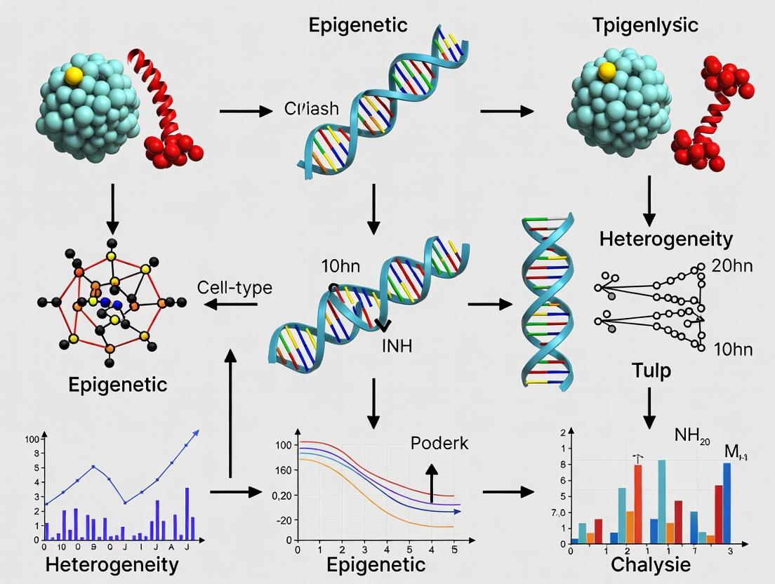
Beyond the Bulk: Decoding Cell-Type Heterogeneity in Epigenetic Analysis for Precision Discovery
This article provides a comprehensive guide for researchers navigating the critical challenge of cell-type heterogeneity in epigenetic studies.
Beyond the Bulk: Decoding Cell-Type Heterogeneity in Epigenetic Analysis for Precision Discovery
Abstract
This article provides a comprehensive guide for researchers navigating the critical challenge of cell-type heterogeneity in epigenetic studies. We begin by defining the problem and its biological significance, explaining how bulk tissue analysis obscures cell-type-specific epigenetic states and can lead to misleading interpretations. We then detail current methodological approaches, from bulk deconvolution algorithms to single-cell and spatial epigenomic technologies, with a focus on practical applications in disease research and drug development. A dedicated troubleshooting section addresses common pitfalls in experimental design, data quality, and computational analysis. Finally, we compare the validation strategies and performance benchmarks for different methodologies. This synthesis equips scientists with the foundational knowledge and practical framework needed to design robust studies, accurately interpret epigenetic data, and drive discoveries in biomedicine.
Why Cell-Type Heterogeneity Matters: The Foundational Challenge in Epigenetics
Technical Support Center
Troubleshooting Guide: Resolving Ambiguity in Epigenetic Data
Q1: Our bulk ATAC-seq data shows high chromatin accessibility at a disease-associated gene locus, but our single-cell follow-up is inconsistent. What could be the issue? A: This is a classic symptom of cellular heterogeneity masking. In bulk analysis, a strong signal can be driven by a small, highly active subpopulation. The average across all cells masks the fact that most cells are inactive.
- Troubleshooting Steps:
- Re-analyze Bulk Data: Apply computational deconvolution tools (e.g., CIBERSORTx, MuSiC) to your bulk data to estimate the proportion of cell types present. This can reveal if a minor population is the signal source.
- Validate with scATAC-seq: Design a targeted single-cell assay. Ensure your cell dissociation protocol is optimized for your tissue type to avoid bias.
- Check Clustering Resolution: In your single-cell analysis, increase the clustering resolution. The relevant subpopulation may be a small cluster that was merged into a larger one.
Q2: When performing bisulfite sequencing on heterogeneous tissue, how do we determine if uniform DNA methylation changes are biologically relevant or an averaging artifact? A: Distinguishing true homogeneity from averaging is critical.
- Troubleshooting Steps:
- Perform Limit Dilution Cloning: After bisulfite conversion, clone PCR amplicons from individual molecules and sequence 10-20 clones. A mix of fully methylated and fully unmethylated clones indicates cellular heterogeneity, while uniformly partially methylated clones suggest true homogeneity.
- Utilize Cell Sorting: Prior to extraction, use FACS to separate major cell types (e.g., by surface markers CD45+, CD31+) and perform bulk analysis on each sorted population.
- Employ Single-Cell Bisulfite Sequencing: If resources allow, use a commercial scBS-seq or snRRBS protocol, acknowledging the current technical limitations in coverage.
Q3: Our ChIP-seq experiment for H3K27ac in a tumor sample yielded broad, weak peaks. How can we clarify if this represents poised enhancers in many cells or active enhancers in a few? A: Broad, weak peaks often suggest a mixed cell state.
- Troubleshooting Steps:
- Co-staining Validation: Perform immunofluorescence (IF) or immunohistochemistry (IHC) on a serial section for H3K27ac and a marker for the suspected active subpopulation. Co-localization supports the subpopulation hypothesis.
- Correlate with scRNA-seq: Integrate existing scRNA-seq data from a similar sample. Check if high expression of your target genes correlates exclusively with a specific cell subtype.
- Optimize ChIP Protocol: Rule out technical causes: perform a spike-in control (e.g., Drosophila chromatin) to normalize for input differences, and titrate antibody concentration to reduce background.
Frequently Asked Questions (FAQs)
Q: What are the primary computational methods to deconvolute bulk epigenetic data? A: Deconvolution requires a reference. Common approaches include:
- Methylation Array Deconvolution: Uses reference methylomes (e.g., from sorted blood cells) to estimate proportions in mixtures. Tools: MethylCIBERSORT, EpiDISH.
- Chromatin Data Deconvolution: Uses cell-type-specific open chromatin or histone mark references (often from public scATAC-seq data). Tools: CIBERSORTx, deconvPeaks.
Q: What are the key trade-offs between single-cell and bulk epigenomic techniques? A:
| Aspect | Bulk Epigenomics | Single-Cell Epigenomics |
|---|---|---|
| Cost per Cell | Very Low | High |
| Genome Coverage | High, Deep | Sparse, Noisy |
| Cell-Throughput | Millions (one measurement) | Thousands (individual profiles) |
| Reveals Heterogeneity | No, Averages | Yes, Directly |
| Primary Use Case | Identifying large-scale, population-level changes | Defining cell states, identifying rare populations, building atlases |
Q: Which single-cell epigenomic technique should I start with to resolve heterogeneity? A: The choice depends on your biological question and sample type:
- scATAC-seq: For mapping chromatin accessibility and inferring transcription factor dynamics across diverse cell types. Best for nuclear samples (frozen tissue).
- snRNA-seq + snmC-seq (multiome): For directly correlating transcriptome and methylome from the same single nucleus. Ideal for brain or complex solid tissues.
- CUT&Tag: For profiling histone modifications (e.g., H3K4me3, H3K27me3) in single cells with lower background than ChIP-based methods.
Experimental Protocols
Protocol 1: Deconvolution of Bulk DNA Methylation Data Using EpiDISH
Purpose: To estimate cell-type proportions from a bulk DNA methylation (e.g., Illumina EPIC array) profile of heterogeneous tissue.
Methodology:
- Input Data Preparation: Format your beta-values matrix (probes x sample). Ensure probe IDs are Illumina CG identifiers.
- Reference Selection: Choose an appropriate reference centroid matrix. For blood tissue, use the
centEpiFibIC.mreference (epithelial, fibroblasts, immune cells). For brain, use a neuron/glia/endothelium reference. - Run Deconvolution: In R, use the
EpiDISHpackage.
- Interpretation: The output
estis a matrix of estimated cell fractions for each sample. Correlate these fractions with your epigenetic signal strength.
Protocol 2: Single-Nucleus Multiome (ATAC + Gene Expression) Assay
Purpose: To simultaneously profile chromatin accessibility and gene expression from the same single nucleus, enabling direct linkage of regulatory elements to cell identity.
Methodology (10x Genomics Chromium Platform):
- Nuclei Isolation: Dounce homogenize flash-frozen tissue in lysis buffer. Filter nuclei through a 40µm flow cell strainer. Stain with DAPI and sort intact nuclei or use a sucrose gradient purification.
- Tagmentation & GEM Generation: Use the Chromium Next GEM Single Cell Multiome ATAC + Gene Expression kit. Nuclei are tagmented with Tn5 transposase, then co-encapsulated with Gel Beads in Emulsion (GEMs) for reverse transcription and ATAC library construction.
- Library Preparation: Perform two separate PCRs: one to amplify the accessible chromatin fragments (ATAC library) and one to amplify the cDNA (Gene Expression library).
- Sequencing & Analysis: Sequence on an Illumina platform (~25k read pairs/nucleus for ATAC, ~10k reads/nucleus for RNA). Use Cell Ranger ARC pipeline for alignment, barcode counting, and peak calling. Subsequent analysis in Signac or ArchR for integrated analysis.
Visualizations
Diagram 1: Bulk vs Single-Cell Epigenetic Analysis Workflow
Diagram 2: Deconvolution of a Bulk Epigenetic Signal
The Scientist's Toolkit: Research Reagent Solutions
| Item | Function in Context of Cellular Heterogeneity |
|---|---|
| 10x Genomics Chromium Single Cell Multiome ATAC + Gene Expression Kit | Enables simultaneous profiling of chromatin accessibility and transcriptome from the same single nucleus, directly linking regulatory landscape to cell identity. |
| Cell Surface Marker Antibody Panels (e.g., for FACS) | Allows physical separation of major cell types from a tissue digest prior to bulk analysis, reducing heterogeneity. Essential for creating reference profiles. |
| Tn5 Transposase (Tagmentase) | Engineered transposase used in ATAC-seq and related methods. Critical for single-cell epigenomics as it integrates tagmentation and library prep in one step. |
| Methylation-Sensitive Restriction Enzymes (e.g., HpaII) | Used in low-input or single-cell methylome techniques like scRRBS to assess DNA methylation heterogeneity at CpG islands. |
| Spike-in Control Chromatin (e.g., Drosophila S2) | Added to ChIP-seq reactions before immunoprecipitation for normalization. Crucial for comparing histone mark signals across heterogeneous samples of varying cell composition. |
| DAPI or Hoechst Stain | Vital for flow cytometry or microscopy-based sorting of intact nuclei from frozen tissues for snATAC-seq or snmC-seq assays. |
| Cell Hashtag Oligonucleotide Antibodies (e.g., BioLegend TotalSeq-A) | Enables sample multiplexing in single-cell experiments. Cells from different conditions are labeled with distinct barcoded antibodies, pooled, and run together, reducing batch effects and costs. |
Technical Support Center: Troubleshooting Guides & FAQs for Epigenomic Profiling
Thesis Context: This support content is designed to address common experimental challenges in the context of resolving cell-type heterogeneity in epigenetic analyses. Accurate interpretation of development, homeostasis, and disease mechanisms hinges on isolating and analyzing pure, well-defined cell populations.
Frequently Asked Questions (FAQs)
Q1: My snATAC-seq data shows high mitochondrial read percentage in nuclei isolated from frozen tissue. What is the cause and solution? A: High mitochondrial reads (>20%) in single-nucleus assays often indicate nuclear membrane damage during isolation or freeze-thaw. This is critical for preserving cell-type-specific chromatin accessibility signals.
- Solution: Optimize the homogenization buffer. Increase the concentration of non-ionic detergent (e.g., NP-40) by 0.1% increments and include 0.1-0.4 U/µl of RNase inhibitor directly in the lysis buffer to protect nuclear RNA. Always use pre-chilled buffers and keep samples on ice.
Q2: In our bulk H3K27ac ChIP-seq from tumor tissue, the signal appears "washed out" and lacks sharp peaks. Could cellular heterogeneity be the issue? A: Yes. A heterogeneous sample containing multiple cell types creates an averaged epigenomic profile, obscuring cell-type-specific enhancer landscapes. This directly confounds the identification of disease-relevant regulatory elements.
- Solution: Prior to ChIP, implement a cell sorting strategy (FACS) using a validated panel of cell surface markers to isolate your target population. If sorting is not feasible, computationally deconvolute the bulk signal using reference single-cell epigenomic datasets (e.g., from CistromeDB) to estimate cell-type contributions.
Q3: After performing CUT&Tag on sorted primary T-cells, the library yield is too low for sequencing. What are the likely troubleshooting steps? A: Low CUT&Tag yield often stems from inefficient permeabilization or antibody penetration.
- Solution: 1) Titrate the digitonin concentration (0.01%-0.1%) during the permeabilization and antibody binding steps. 2) Ensure the Concanavalin A-coated beads are fresh and thoroughly washed. 3) Increase the number of input cells to 50,000-100,000 for low-abundant cell types. Verify antibody suitability for CUT&Tag using published data.
Q4: How can we validate that an epigenetic modifier drug is acting on a specific cell type in a complex co-culture system? A: This requires a method to capture the epigenome with cell-type identification.
- Solution: Implement a CUT&Tag or scATAC-seq workflow with integrated cell hashing. Label each cell population in co-culture with a unique lipid-tagged or antibody-tagged barcode (e.g., TotalSeq). After epigenomic profiling, demultiplex the data to assign epigenetic changes to the correct cell type, directly testing cell-type-specific drug action.
Q5: Our scRNA-seq data from a developing organ shows distinct clusters, but how can we link these transcriptional states to changes in the regulatory landscape? A: This requires multi-omic integration.
- Solution: Perform a multiome assay (e.g., 10x Multiome ATAC + Gene Expression) on the same single cell. Alternatively, use computational tools like Signac or ArchR to integrate paired scRNA-seq and snATAC-seq datasets from analogous samples, linking open chromatin regions to putative target genes and transcription factors driving cell fate.
Experimental Protocol: snATAC-seq on Frozen Human Tissue Sections
This protocol is optimized for preserving cell-type-specific chromatin accessibility.
I. Nuclei Isolation from Frozen Tissue
- Cryopreserved Tissue Pulverization: Place 20-50 mg frozen tissue in a chilled Covaris tissue bag. Pulverize using the CryoPREP system (3 cycles, impact level 4). Keep powder frozen in liquid nitrogen.
- Homogenization: Transfer powder to a Dounce homogenizer with 2 ml of Nuclei EZ Lysis Buffer (Sigma NUC101) supplemented with 0.1% NP-40, 0.2 U/µl RNase Inhibitor, and 1x EDTA-free protease inhibitor. Dounce 15-20 times with the "loose" pestle (A), then 10-15 times with the "tight" pestle (B) on ice.
- Filtration & Centrifugation: Filter homogenate through a 40 µm Flowmi cell strainer. Incubate on ice for 5 min. Centrifuge at 500g for 5 min at 4°C.
- Wash & Count: Gently resuspend pellet in 1 ml of Wash & Resuspension Buffer (1x PBS, 1% BSA, 0.2 U/µl RNase Inhibitor, 0.1% Tween-20). Centrifuge at 500g for 5 min at 4°C. Resuspend in 100 µl of the same buffer. Count nuclei using AO/PI staining on a LUNA-FL or hemocytometer. Aim for viability >85%.
II. Tagmentation with Tn5 (10x Genomics Compatible)
- Dilute nuclei to 1000 nuclei/µl in Wash & Resuspension Buffer.
- For 10,000 nuclei, combine in a nuclease-free tube:
- 10 µl nuclei (10,000 nuclei)
- 10 µl Tagmentation Buffer (10x Genomics, 20005778)
- 8.5 µl nuclease-free water
- 1.5 µl Assay Buffer (10x Genomics, 20005779)
- Mix gently and incubate at 37°C for 60 min in a thermomixer with gentle shaking (300 rpm).
- Immediately add 50 µl of SB Buffer (from 10x kit) and mix. Proceed to nuclei cleanup with provided beads per manufacturer's instructions.
III. Library Preparation & Sequencing
- Perform PCR amplification of tagmented DNA using indexed primers (10x kit). Determine cycle number using qPCR side reaction or manufacturer's guidelines (typically 12-14 cycles).
- Clean up libraries with SPRIselect beads (0.6x right-side size selection, followed by 1.2x left-side selection).
- Assess library quality on a Bioanalyzer (High Sensitivity DNA chip). Expect a nucleosomal periodicity pattern (∼200 bp ladder).
- Sequence on an Illumina platform. Recommended depth: 20,000-50,000 reads per nucleus for human/mouse. Use paired-end sequencing (e.g., PE50).
Data Presentation
Table 1: Common Epigenomic Assays and Their Suitability for Heterogeneous Samples
| Assay | Input Material | Cell-Type Resolution | Key Output | Major Challenge for Heterogeneous Tissues |
|---|---|---|---|---|
| Bulk ChIP-seq | Cross-linked cells/tissue | None - Averages signal | Protein-DNA binding sites (e.g., H3K27ac) | Signal convolution from multiple cell types; requires prior sorting. |
| Bulk ATAC-seq | Live cells/nuclei | None - Averages signal | Genome-wide chromatin accessibility | Identifies accessible regions but cannot assign them to a specific cell type. |
| CUT&Tag | Permeabilized cells | Low (if sorted) | Protein-DNA binding sites | Low input is possible but best performed on pre-sorted populations. |
| snATAC-seq | Isolated nuclei | High - Single nucleus | Cell-type-specific chromatin accessibility | Nuclear isolation must be optimized to avoid loss of fragile nuclei types. |
| scChIC-seq | Single cells | High - Single cell | Histone modification states in single cells | Technically challenging; low throughput. |
| Multiome (ATAC + GEX) | Isolated nuclei | High - Single nucleus | Paired accessibility and transcriptome | Premium cost; complex data analysis. |
Table 2: Troubleshooting Metrics for snATAC-seq Quality Control
| QC Metric | Optimal Range | Warning Range | Indicated Problem | Corrective Action |
|---|---|---|---|---|
| Nuclei Viability (AO/PI) | >85% | 70-85% | Excessive lysis/damage | Optimize homogenization; add RNase inhibitor. |
| Median Fragments/Nucleus | 20,000 - 50,000 | <10,000 | Inefficient tagmentation | Titrate Tn5 enzyme; check nuclei integrity. |
| Fraction of Fragments in Peaks | 30-60% | <20% | High background | Increase PCR cycles; check Tn5 activity. |
| TSS Enrichment Score | >10 | <6 | Low signal-to-noise | Improve nuclei quality; ensure fresh reagents. |
| Mitochondrial Read % | <10% | >20% | Nuclear damage | Gentler homogenization; optimize lysis buffer. |
The Scientist's Toolkit: Research Reagent Solutions
| Item | Function in Epigenetic Analysis | Example Product/Catalog # |
|---|---|---|
| Concanavalin A Beads | Binds to glycoproteins on nuclear membrane for immobilization during CUT&Tag. | Bruker CUT&Tag Beads (Bruker, 21485) |
| Tn5 Transposase | Engineered transposase that simultaneously fragments ("tags") DNA and adds sequencing adapters in ATAC-seq. | Illumina Tagment DNA TDE1 Enzyme (20034197) |
| Digitonin | Mild, cholesterol-dependent detergent for cell permeabilization in CUT&Tag and intracellular antibody staining. | MilliporeSigma (D141) |
| Nuclei Isolation Buffer | A refined, osmotically balanced buffer for extracting intact nuclei from difficult or frozen tissues. | Nuclei EZ Lysis Buffer (Sigma, NUC101) |
| Cell Hashing Antibodies | Antibodies conjugated with unique oligonucleotide barcodes to label cell populations for multiplexing and doublet detection. | BioLegend TotalSeq-A Antibodies |
| SPRIselect Beads | Size-selective magnetic beads for post-tagmentation cleanup and library size selection. | Beckman Coulter, B23318 |
| RNase Inhibitor | Protects nuclear RNA during isolation, crucial for maintaining nuclear integrity in snATAC-seq. | Protector RNase Inhibitor (Sigma, 3335402001) |
| DAPI (AO/PI) | Vital dyes for staining and quantifying DNA to assess nuclei integrity and count. | Acridine Orange/Propidium Iodide (Logos Biosystems, F23001) |
Visualizations
Title: snATAC-seq Experimental Workflow from Tissue to Data
Title: Resolving Cell-Type-Specific Signals from Heterogeneous Tissues
Title: Multi-omic Data Integration Workflow for Cell States
Troubleshooting Guides & FAQs
Q1: Our bulk ATAC-seq data shows inconsistent epigenetic marks between biological replicates from the same tissue. What could be the cause? A: This is frequently caused by variability in cellular composition between samples. Even small shifts in the proportion of constituent cell types can drastically alter bulk signal averages. First, validate composition using:
- Flow cytometry with a panel of canonical surface markers.
- Reference-based deconvolution of your sequencing data (e.g., using CIBERSORTx, MuSiC) against a validated, cell-type-specific epigenetic signature matrix.
Q2: After sorting a specific cell population for ChIP-seq, we still detect marks associated with other cell types. Are the assays contaminated? A: Not necessarily. This often represents the 'Averaging' Artifact at a higher resolution. "Pure" populations defined by 2-3 surface markers often contain transcriptional subtypes with distinct epigenomes. Consider:
- Increasing resolution: Use single-cell ATAC-seq (scATAC-seq) or CUT&Tag on the sorted population.
- Re-evaluating sorting gates: Include additional markers to exclude closely related subtypes.
- Bioinformatic correction: Apply computational tools like Feature Barcoding-based deconvolution in single-cell analysis.
Q3: How significant can the effect of cellular composition be on a bulk DNA methylation (e.g., WGBS) signal? A: The effect is substantial. A shift of 10% in a minor cell population with a strong differentially methylated region (DMR) can change the bulk beta value by 0.1, which is often interpreted as a biologically significant finding.
Table 1: Impact of Cellular Composition Shift on Bulk Epigenetic Signal
| Assay | Composition Change | Potential Signal Change | Common Misinterpretation |
|---|---|---|---|
| Bulk ATAC-seq | ±15% of a rare immune cell type | Peak height change >2-fold at cell-type-specific enhancers | Erroneous conclusion of global chromatin accessibility shift. |
| Bulk H3K27ac ChIP-seq | ±10% of a progenitor cell population | False-positive "gained" signal at progenitor-specific genes. | Misidentification of active regulatory elements. |
| Bulk WGBS | ±20% of a stromal cell type | Methylation beta value shift of 0.15-0.2 at DMRs. | Incorrect attribution of hypo/hypermethylation to main cell type. |
Q4: What is the best experimental design to avoid the averaging artifact? A: The optimal approach is a tiered, multi-resolution strategy:
- Initial Discovery: Perform high-depth single-cell multiomics (e.g., scATAC-seq + scRNA-seq) on a representative set of unsorted samples to define the complete cellular atlas and its epigenetic states.
- Targeted Validation: Use fluorescence-activated nucleus sorting (FANS) or antibody-based TAMe-ChIP to isolate nuclei/cells based on specific chromatin features or markers identified in step 1 for lower-noise, population-targeted assays.
- Functional Studies: Employ perturbation-based assays (e.g., EpiTOF, CUT&Run after CRISPRi) in sorted populations to establish causality.
Detailed Methodologies
Protocol: Cell-Type-Specific Deconvolution of Bulk DNA Methylation Data
- Generate a Reference Matrix:
- Isulate pure cell populations (>99% by FACS) of all major constituent types (n≥5 per type).
- Perform reduced representation bisulfite sequencing (RRBS) or EPIC array on each.
- Identify cell-type-specific differentially methylated CpGs (csDMCs) (ANOVA, adj. p < 0.01, Δβ > 0.5).
- Create a matrix of mean methylation β-values at these csDMCs for each pure type.
- Deconvolute Bulk Samples:
- Process your bulk WGBS/RRBS data.
- Extract β-values for the csDMCs defined in your reference.
- Use a constrained least squares regression method (e.g., projectCellType from the minfi R package) to estimate the proportion of each cell type in each bulk sample.
- Statistical Adjustment:
- Include the estimated proportions as covariates in downstream differential methylation analysis to distinguish true epigenetic changes from composition-driven artifacts.
Protocol: Single-Cell ATAC-seq (scATAC-seq) for Heterogeneity Analysis
- Nuclei Isolation & Tagmentation: Isolate nuclei from fresh or frozen tissue using a gentle lysis buffer. Perform tagmentation using the Tn5 transposase (e.g., from the 10x Genomics Chromium Next GEM kit).
- Barcoding & Library Prep: Use a microfluidic system to partition single nuclei into Gel Beads in Emulsion (GEMs). Each bead contains a unique barcode to label all chromatin fragments from the same nucleus. Perform PCR amplification.
- Sequencing & Analysis: Sequence on an Illumina platform (paired-end). Process data using Cell Ranger ARC. Perform dimensionality reduction (LSI), clustering (Louvain), and integration with matched scRNA-seq data via WNN in Seurat to annotate cell types and link accessible chromatin to transcriptional states.
Visualizations
Bulk Analysis Creates Averaging Artifact
scATAC-seq Workflow for Deconvolution
The Scientist's Toolkit: Research Reagent Solutions
Table 2: Essential Reagents for Resolving Epigenetic Heterogeneity
| Item | Function | Example Product/Catalog |
|---|---|---|
| 10x Chromium Next GEM Chip J | Microfluidic chip for partitioning single nuclei/cells into barcoded droplets for scATAC-seq or multiome assays. | 10x Genomics, 1000230 |
| Tn5 Transposase (Loaded) | Enzyme that simultaneously fragments ("tagments") chromatin and adds sequencing adapters. Critical for ATAC-seq. | Illumina Tagment DNA TDE1 Enzyme, 20034197 |
| Cell-Surface Marker Antibody Panel | Antibodies for fluorescence-activated cell sorting (FACS) to isolate pure populations for reference generation. | BioLegend TotalSeq-C antibodies for CITE-seq |
| Nuclei Isolation Kit | Gentle, non-ionic detergent-based buffers to extract intact nuclei from complex tissues for epigenetics. | 10x Genomics Nuclei Isolation Kit, 1000494 |
| Methylation-Sensitive Restriction Enzymes | For enzymatic methyl-seq approaches or validating DMRs (e.g., HpaII, McrBC). | NEB HpaII, R0171S |
| SPRIselect Beads | Size-selective magnetic beads for post-tagmentation clean-up and library size selection in NGS prep. | Beckman Coulter, B23318 |
| PMA (Prolonged Methylation Agent) | Chemical for in vitro methylation of DNA to serve as a spike-in control for WGBS efficiency. | Sigma-Aldrich, M0251 |
Epigenetic Analysis Technical Support Center
Welcome. This center provides support for researchers navigating the technical challenges of epigenetic analysis, with a specific focus on mitigating misinterpretation arising from unaccounted cell-type heterogeneity. The following guides address common pitfalls in major disease areas.
Troubleshooting Guides & FAQs
Q1: In our cancer methylation study, we observe widespread hypermethylation. Could this be a technical artifact rather than a true biological signal? A: This is a frequent concern. The observed signal may be driven by shifts in the tumor microenvironment (e.g., changes in stromal, immune, or endothelial cell proportions) rather than epigenetic change within malignant cells.
- Troubleshooting Steps:
- Deconvolution Check: Run a reference-based deconvolution tool (e.g., CIBERSORTx, EpiDISH) using an appropriate cancer-specific reference. Quantify the estimated cell-type proportions.
- Correlation Analysis: Correlate the degree of hypermethylation at key loci with the estimated proportion of stromal cells. A high positive correlation suggests a confounding effect.
- Validation Experiment: Perform immunofluorescence or flow cytometry on a matched sample subset for canonical markers (e.g., α-SMA for cancer-associated fibroblasts, CD45 for leukocytes). Compare with deconvolution estimates.
Q2: When analyzing bulk histone modification ChIP-seq data from post-mortem brain tissue, how do we dissect contributions from neurons versus glia? A: Neurological studies are highly susceptible to misinterpretation due to the complex and variable cellular composition of brain regions.
- Troubleshooting Steps:
- Sequencing Depth Audit: Ensure sufficient sequencing depth (>50 million non-duplicate reads for bulk H3K27ac ChIP-seq) to detect signals from minority cell populations.
- In-Silico Separation: Use tools like
brainimmuneorBRETIGEAto estimate neuronal, astrocyte, microglial, and oligodendrocyte content from RNA-seq data of the same samples. Statistically adjust the ChIP-seq peak intensities using these estimates as covariates. - Wet-Lab Validation: If feasible, perform H3K9me3 or H3K4me3 ChIP-seq on fluorescence-activated nuclei sorting (FANS)-isolated NeuN+ (neuronal) and NeuN- (non-neuronal) nuclei from replicate tissue.
Q3: In PBMC epigenomic studies of autoimmune disease, our differential analysis identifies vast numbers of ATAC-seq peaks. How do we prioritize peaks specific to a rare immune subset? A: Bulk analysis of PBMCs often reflects dominant cell types (e.g., T cells), masking signals from rare but pathogenic subsets (e.g., T follicular helper cells).
- Troubleshooting Steps:
- Proportion-Aware Analysis: Use a differential analysis method designed for compositional data (e.g.,
LinDA,ANCOM-BC) that accounts for the simplex nature of cell proportions. - Peak Deconvolution: Employ a tool like
TOBIASwith a leukocyte epigenome atlas to estimate the contribution of specific immune cell types to each differentially accessible peak. - Focus on Subset-Signature Peaks: Intersect your differential peaks with publicly available ATAC-seq or ChIP-seq peaks from purified immune subsets (e.g., from DICE or Blueprint projects). Prioritize peaks unique to the disease-relevant subset.
- Proportion-Aware Analysis: Use a differential analysis method designed for compositional data (e.g.,
Q4: For complex diseases like fibrosis or atherosclerosis, how do we determine if epigenetic changes are cause or consequence of cellular composition changes? A: This is a fundamental challenge. The observed "epigenetic shift" may simply be the presence of a new cell type.
- Troubleshooting Steps:
- Longitudinal/Experimental Design: If possible, analyze serial samples from a disease model to track epigenetic and cellular changes over time.
- Single-Cell Validation: Perform pilot snATAC-seq or scChIC-seq on a subset of samples. This directly assays chromatin state with cell identity.
- Causal Inference Modeling: Apply computational frameworks like
ICELLNETor cell–cell communication inference to snRNA-seq data to predict signaling pathways that may be inducing epigenetic changes in recipient cells, generating hypotheses for mechanistic validation.
Detailed Experimental Protocol: Cell-Type Deconvolution-Adjusted Epigenome-Wide Association Study (EWAS)
Objective: To identify DNA methylation differences associated with a phenotype (e.g., disease status) after statistically controlling for variation in cell-type composition.
Materials:
- Input Data: Bulk DNA methylation array data (IDAT files or beta/matrix).
- Software: R (v4.2+),
minfi,EpiDISH,sva,limmapackages. - Reference Matrix: A pre-defined reference matrix of cell-type-specific methylation signatures (e.g.,
centEpiFibIC.mfor EpiDISH, containing centroids for epithelial, fibroblasts, and immune cells).
Methodology:
- Data Preprocessing: Load IDAT files with
minfi. Perform quality control (detection p-value > 0.01), normalization (e.g., functional normalization), and probe filtering (remove cross-reactive and SNP-containing probes). - Cell Proportion Estimation: Using the
EpiDISHpackage, apply theepidish()function with theRPC(Robust Partial Correlation) method and your chosen reference matrix to estimate cell proportions for each sample. - Covariate Adjustment: Create a design matrix for linear modeling. Crucially, include the estimated cell proportions (e.g., Fibroblast %, Immune Cell %) as continuous covariates alongside the primary variable of interest (e.g., Disease vs. Control) and other technical covariates (Batch, Age, Sex).
- Differential Methylation Analysis: Use the
limmapackage to fit the linear model and perform an empirical Bayes moderation. Extract significantly differentially methylated CpG sites (e.g., FDR-adjusted p-value < 0.05, delta-beta > 0.1). - Sensitivity Analysis: Re-run the analysis without cell proportion covariates. Compare the lists of significant hits. Probes that disappear after adjustment were likely confounded by cellular heterogeneity.
Table 1: Impact of Cell-Type Correction on Differential Methylation Findings in a Simulated Colorectal Cancer Dataset
| Analysis Method | Total Significant CpGs (FDR<0.05) | CpGs Unique to Method | Overlap with Known Cancer-Specific CpGs* |
|---|---|---|---|
| Standard EWAS (No Correction) | 12,450 | 8,211 | 45% |
| EWAS with Cell Proportion Covariates | 5,877 | 1,638 | 92% |
| Overlap Between Methods | 4,239 | - | 98% |
*Based on comparison with independent single-cell methylome data from purified colon epithelial cells.
Table 2: Common Deconvolution Tools for Epigenetic Data
| Tool Name | Primary Application | Required Input | Key Output | Considerations |
|---|---|---|---|---|
| CIBERSORTx | RNA-seq, Methylation | Bulk profile, Signature matrix (GEP/LMG) | Cell fractions, Imputed profiles | High accuracy, needs a robust custom signature. |
| EpiDISH | DNA Methylation | Bulk beta/m-values, Reference centroid matrix | Cell proportion estimates | Fast, has built-in references for blood, epithelia, etc. |
| MuSiC | RNA-seq | scRNA-seq reference, Bulk RNA-seq | Cell-type proportions | Leverages single-cell reference, good for closely related types. |
| TOBIAS | ATAC-seq/ChIP-seq | Bulk ATAC-seq peaks, Footprint reference | Corrected footprint scores, Cell-type activity | Directly models TF binding, computationally intensive. |
Pathway & Workflow Visualizations
Title: Correct vs. Incorrect Paths in Heterogeneous Tissue Analysis
Title: Deconvolution-Adjusted EWAS Workflow
Title: Example: Immune Signaling to Epigenetic Change in Stroma
The Scientist's Toolkit: Key Research Reagent Solutions
| Item | Function & Relevance to Heterogeneity |
|---|---|
| 10x Genomics Chromium Single Cell ATAC | Enables high-throughput profiling of chromatin accessibility in single nuclei, directly measuring epigenomic heterogeneity. |
| Fluorescence-Activated Nuclei Sorting (FANS) Antibodies (e.g., Anti-NeuN, Anti-SOX10) | Allows physical isolation of specific cell-type nuclei from frozen tissue for bulk epigenomic assays, reducing heterogeneity. |
| MethylationEPIC v2.0 BeadChip Array | Provides genome-wide CpG coverage. Use with deconvolution algorithms (EpiDISH) to estimate cell proportions from bulk tissue. |
| CUT&Tag Assay Kits (e.g., for H3K27ac) | A low-input, high-signal alternative to ChIP-seq. Enables histone mark profiling from FANS-sorted or limited cell populations. |
| Validated Reference Epigenome Sets (e.g., BLUEPRINT, Roadmap) | Provide essential cell-type-specific reference methylomes or chromatin states required for accurate in-silico deconvolution. |
| Nuclei Isolation & Lysis Buffers (for snATAC/RNA) | Critical first step for single-nucleus epigenomics from complex solid tissues (brain, tumor). Quality dictates library complexity. |
Technical Support Center
Troubleshooting Guides & FAQs
Q1: During single-cell ATAC-seq analysis, my cluster markers show high heterogeneity, and I cannot clearly define distinct cell types. Is this a failure? A: Not necessarily. This "failure" is an opportunity. High intra-cluster heterogeneity can reveal substates, dynamic transitions, or novel subpopulations. First, ensure your bioinformatics pipeline is robust.
- Check: Are you using appropriate batch correction (e.g., Harmony, Seurat's CCA integration) for technical variation?
- Reframe: Instead of forcing more clusters, perform trajectory inference (e.g., with Monocle3, PAGA) on the heterogeneous cluster to see if it represents a continuum of differentiation or activation states.
Q2: My bulk ChIP-seq data for a histone mark shows an intermediate, "smudged" signal profile. What does this mean? A: An intermediate, broad signal in bulk analysis is a classic signature of cell-type or state heterogeneity within your sample.
- Troubleshooting Step: Quantify the proportion of cells expected to bear the mark. Use this table to interpret your signal:
| Observed Bulk Signal Profile | Possible Biological Interpretation | Recommended Action |
|---|---|---|
| Sharp, defined peaks | Homogeneous cell population or synchronized state. | Proceed with standard analysis. |
| Broad, "smudged" enrichment | Mixed cell populations with varying mark levels. | Perform deconvolution analysis (e.g., with CIBERSORTx, MuSiC) using a single-cell reference. |
| Very low or noisy signal | Target mark is present in only a rare subpopulation. | Shift to single-cell or single-nucleus assay (snATAC-seq/ChIP-seq). |
Q3: When validating a candidate drug target in a cell line model, response is highly variable between replicates. Could heterogeneity be the cause? A: Yes. Even canonical cell lines contain subpopulations with differential epigenetic priming, leading to divergent drug responses.
- Protocol: Identifying Resistant Subpopulations via H3K27ac ChIP-seq:
- Treat your cell population with the drug at IC50.
- After 72 hours, separate viable (resistant) from non-viable (sensitive) cells using FACS or a viability dye.
- Perform H3K27ac ChIP-seq on both the resistant and parental (untreated) populations.
- Compare enhancer landscapes. Resistant subpopulations often show pre-existing, heightened activity at enhancers near pro-survival or alternative pathway genes.
- Validate by sorting the top 10% of cells expressing the gene from that enhancer before treatment and confirm higher survival rates.
The Scientist's Toolkit: Research Reagent Solutions
| Item | Function in Heterogeneity Analysis |
|---|---|
| 10x Genomics Chromium Controller | Enables high-throughput single-cell/nucleus library generation for ATAC-seq, multiome (ATAC + GEX). Essential for capturing heterogeneity. |
| Tn5 Transposase (Tagmentase) | Engineered transposase that simultaneously fragments and tags chromatin DNA for ATAC-seq. Batch consistency is critical for reproducibility. |
| Methylase (e.g., M.CviPI) | Used in NOME-seq and SMAC-seq protocols to mark accessible DNA (GpC methylation), providing a footprint of nucleosome positions and TF occupancy within heterogeneous samples. |
| Cell Hashing Antibodies (TotalSeq) | Allows sample multiplexing by tagging cells from different conditions with unique lipid-tagged antibodies, reducing batch effects and enabling cleaner comparison of subpopulations across conditions. |
| ATAC-seq Enhancer (CRISPRa) Perturb-seq Pools | Combines epigenetic perturbation (dCas9-p300) with single-cell readout to functionally link candidate regulatory elements to genes and phenotypes in a heterogeneous pool of perturbations. |
Experimental Protocols
Protocol: Single-Nucleus Multiome (ATAC + Gene Expression) for Complex Tissues Objective: To simultaneously profile chromatin accessibility and transcriptome from the same nucleus in a frozen tissue sample, resolving cellular heterogeneity and linking regulators to genes.
- Nuclei Isolation: Dounce homogenize 25mg frozen tissue in chilled lysis buffer (10mM Tris-HCl pH7.4, 10mM NaCl, 3mM MgCl2, 0.1% Tween-20, 0.1% NP-40, 0.01% Digitonin, 1U/μL RNase inhibitor). Filter through a 40μm flowmi strainer.
- Nuclei Sorting & Counting: Stain with DAPI and sort using FACS for intact, single nuclei. Count with hemocytometer. Target viability >90%.
- 10x Multiome Library Preparation: Use the 10x Genomics Chromium Next GEM Single Cell Multiome ATAC + Gene Expression kit. Follow kit protocol to:
- Perform tagmentation on nuclei with loaded Tn5.
- Partition nuclei into Gel Beads-in-emulsion (GEMs).
- Perform GEM-RT for cDNA synthesis and pre-amplification.
- Break emulsions and purify DNA/RNA.
- Library Construction: Generate separate ATAC and Gene Expression libraries via PCR amplification with indexed primers.
- Sequencing: Sequence on Illumina NovaSeq. Recommended: ATAC library: 50k paired-end reads/nucleus; GEX library: 25k reads/nucleus.
- Bioinformatic Analysis: Process with Cell Ranger ARC. Use ArchR or Signac for downstream integrative analysis, clustering, and motif enrichment.
Protocol: CUT&RUN for Low-Input Histone Mark Profiling in Sorted Subpopulations Objective: To map histone modifications from rare cell subpopulations (e.g., 10k-50k cells) isolated by FACS with high signal-to-noise.
- Cell Preparation: Fix sorted cells lightly with 0.1% formaldehyde for 2 minutes at room temperature. Quench with 125mM Glycine.
- Permeabilization & Binding: Permeabilize cells with Digitonin. Bind to pre-activated Concanavalin A-coated magnetic beads.
- Antibody Incubation: Incubate bead-bound cells overnight at 4°C with 1-3μg of primary antibody against target histone mark (e.g., H3K27me3).
- pA-MNase Binding & Cleavage: Wash, then incubate with Protein A-Micrococcal Nuclease (pA-MNase) fusion protein for 1hr at 4°C. Activate MNase by adding CaCl₂ to 2mM final concentration for 30 minutes on ice.
- DNA Extraction: Stop reaction with EGTA. Release DNA fragments from beads by heating with Proteinase K and SDS. Extract with Phenol-Chloroform and precipitate.
- Library Prep & Sequencing: Prepare sequencing library using NEBNext Ultra II DNA kit. Size select for fragments 100-500bp. Sequence single-end 50bp on HiSeq 4000.
Visualizations
Title: From Sample to Discovery: Two Analytical Paths
Title: Epigenetic Heterogeneity Drives Differential Drug Response
Navigating the Toolkit: Methods to Resolve Epigenetic Heterogeneity
Technical Support Center
Troubleshooting Guides & FAQs
Q1: My deconvolution algorithm for ATAC-seq data consistently fails to converge, returning highly variable cell-type proportion estimates between runs. What could be the cause? A: This is often caused by insufficient marker region selection or high multicollinearity in the reference signature matrix. Ensure your reference is built from pure cell types with distinct, open chromatin profiles. Use algorithms like CIBERSORTx or MethylCIBERSORT in high-throughput mode with 500-1000 permutations. Increase the number of marker peaks (we recommend >500 per cell type) to improve condition number. Pre-filter peaks with low variability (variance < 0.1 across reference samples) before matrix construction.
Q2: When deconvoluting DNA methylation array data (e.g., Illumina EPIC), how do I handle probes that are polymorphic or cross-reactive? A: Cross-reactive probes can severely bias estimates. Follow this protocol:
- Download the latest probe exclusion list from the University of California, San Francisco (UCSF) or Zhou et al. (Nucleic Acids Research, 2024).
- Remove all probes listed as polymorphic (SNP at CpG or single-base extension site) or having ≥ 47-base homology to multiple genomic locations.
- Apply a detection p-value threshold of 0.01; fail samples where >5% of probes exceed this threshold.
- Use a reference-based algorithm like EpiDISH or MethylResolver which incorporates these filtering steps internally. See Table 1 for a quantitative summary of recommended probes for deconvolution.
Q3: For histone mark ChIP-seq data deconvolution, what is the optimal strategy for handling input control and peak calling variability? A: Do not use peak-called binary data. Use quantitative signal measurements (e.g., reads per kilobase per million (RPKM) or counts in pre-defined genomic bins). Generate a consensus peak set across all pure cell type reference samples using MACS2 or SPP with a stringent FDR (e.g., 0.01). Extract signal for this consensus set in all samples. Normalize using the input control via methods like csaw or DiffBind. For deconvolution, ChIPDeconv or PREDE are specifically designed for this continuous, normalized input.
Q4: How can I validate my deconvolution results in the absence of physical cell sorting? A: Employ a multi-modal consistency check protocol:
- Cross-platform validation: If deconvoluting ATAC-seq data, compare proportions with those derived from paired RNA-seq (using CIBERSORTx) or DNAm from the same bulk sample.
- Physical mixture reconstruction: Artificially mix pure cell line epigenomic data in known proportions (e.g., 30/70, 50/50) and run your deconvolution pipeline. Accuracy is measured by Root Mean Square Error (RMSE). See Table 2 for performance metrics of popular tools.
- Spatial correlation: If tissue location is available, correlate deconvoluted proportions of known spatially-restricted cell types (e.g., glomerular cells) with their expected histological location.
Q5: My reference matrix is missing a rare but biologically critical cell type (<2% abundance). Can I still deconvolute it accurately? A: Detection of rare cell types is challenging. You must:
- Ensure the reference signature for the rare cell type is derived from highly pure, replicated samples and exhibits strong, unique epigenetic marks (e.g., super-enhancers for ATAC-seq, hypomethylated blocks for DNAm).
- Use a digitally reconstructed rare cell type profile by subtracting major population signals if a physical pure sample is unavailable (feature available in CIBERSORTx).
- Apply a bootstrap approach (n>100) to estimate confidence intervals for the rare population proportion. Report results only if the lower CI is >0.5% and the signature is stable across bootstrap iterations.
Experimental Protocols
Protocol 1: Constructing a DNA Methylation Deconvolution Reference Matrix from Public Data
- Source Data: Download IDAT files and phenotype data for pure cell types (e.g., from Blueprint Epigenome or Gene Expression Omnibus).
- Preprocessing: Process all arrays through minfi (R package) with Noob background correction and dye-bias normalization. Annotate to hg38.
- Probe Filtering: Remove probes with detection p-value > 0.01 in any sample, non-CpG probes, SNP-related probes, and XY chromosomes.
- Beta-value Calculation: Calculate methylation beta-values (M/(M+U+100)).
- DMR Selection: For each cell type pair, identify differentially methylated regions (DMRs) using DSS or limma (absolute delta-beta > 0.4, adjusted p-value < 0.001).
- Matrix Compilation: For each cell type, take the top 500 most hypermethylated and top 500 most hypomethylated DMRs (by delta-beta) versus all others. Calculate the average beta-value within each DMR for each reference sample to build the final M (cell types) x N (DMRs) matrix.
Protocol 2: Bulk ATAC-seq Deconvolution Using a Pre-defined Signature
- Bulk Sample Processing: Sequence bulk ATAC-seq (standard protocol). Align to reference genome (hg38) using BWA-mem2. Call peaks using MACS2 with parameters
--nomodel --shift -100 --extsize 200. - Reference Matrix Loading: Load your pre-constructed cell-type-specific ATAC-seq peak reference matrix (format: peaks x cell types).
- Peak Intersection: Take the intersection of peaks present in both the bulk sample and the reference matrix.
- Deconvolution Execution: Run the LSFit or quadratic programming solver (e.g., via MuSiC package in R). Use the following core command:
- Output Analysis: The
results$Est.propcontains the estimated cell-type proportions. Perform 100 bootstrap iterations on the peak set to estimate standard errors.
Table 1: Recommended Probe/Region Counts for Stable Reference Matrices
| Data Type | Platform/Tool | Minimum Recommended Features per Cell Type | Typical RMSE in Reconstructions | Key Filtering Criteria |
|---|---|---|---|---|
| DNA Methylation | Illumina EPIC Array | 800-1200 DMRs | 0.02 - 0.05 | Delta-beta > 0.4, Adj. p-val < 0.001, no SNPs |
| ATAC-seq | Bulk Sequencing | 500-1000 Peaks | 0.03 - 0.07 | FDR < 0.01, Fold-Change > 2, RPKM > 5 in pure |
| Histone Marks | ChIP-seq (H3K27ac) | 1000-2000 Enhancer Regions | 0.04 - 0.09 | FDR < 0.01, Counts > 20, Input Normalized |
Table 2: Performance Comparison of Major Deconvolution Algorithms (Synthetic Mixtures)
| Algorithm Name | Primary Data Type | Reported Median Correlation (r) | Median RMSE | Computational Speed (per sample) | Recommended Use Case |
|---|---|---|---|---|---|
| CIBERSORTx | RNA-seq, ATAC-seq | 0.95 | 0.02 | Medium (requires offline upload) | High-accuracy, well-defined reference |
| EpiDISH | DNA Methylation | 0.92 | 0.04 | Fast | Array-based DNAm, 3-7 cell types |
| MethylResolver | DNA Methylation | 0.96 | 0.03 | Slow | Complex mixtures (>10 cell types) |
| MuSiC | RNA-seq, ATAC-seq | 0.90 | 0.05 | Fast | Large reference panels (single-cell) |
| PREDE | Histone Mark ChIP-seq | 0.88 | 0.06 | Medium | Quantitative ChIP-seq signal deconvolution |
Diagrams
Title: Bulk Tissue Deconvolution Core Workflow
Title: Data-Specific Deconvolution Pathway
The Scientist's Toolkit: Research Reagent Solutions
| Item/Category | Function in Deconvolution Experiments |
|---|---|
| Pure Cell Type Epigenomic Reference Kits (e.g., EpiCypher's CUT&RUN Reference Sets) | Provides validated, high-quality epigenomic profiles from purified primary cells for building accurate signature matrices. |
| Methylated & Unmethylated DNA Control Standards (e.g., Zymo Research's EZ DNA) | Essential for normalizing DNA methylation arrays (Illumina EPIC/850K) and assessing assay performance in reference generation. |
| Tn5 Transposase (Tagmentase) | For consistent ATAC-seq library preparation from low-input pure cell populations and bulk tissues to minimize batch effects. |
| Histone Modification Specific Antibodies (e.g., Active Motif, Abcam) | High-specificity, ChIP-grade antibodies are critical for generating clean histone mark reference profiles for deconvolution. |
| Cell Surface Marker Antibody Panels (for Sorting) | To isolate pure cell populations via FACS prior to reference epigenomic profiling (e.g., CD45+, CD3+, CD19+ for immune cells). |
| Spike-in Control Chromatin (e.g., Drosophila S2 chromatin) | For normalizing ChIP-seq and ATAC-seq signals across batches during reference generation, improving cross-lab reproducibility. |
| DNA Methylation Spike-ins (e.g., SRA Methylated Plasmid Controls) | To monitor bisulfite conversion efficiency and sequencing coverage uniformity in DNA methylation deconvolution workflows. |
| Computational Tools Suite (R/Bioconductor: minfi, EpiDISH, MuSiC, ChIPDeconv) | Open-source software packages specifically designed for preprocessing and deconvolution of bulk epigenomic data. |
Technical Support Center
This support center provides troubleshooting guidance for single-cell epigenetic assays, framed within the critical research thesis of understanding cell-type heterogeneity in epigenetic analysis. Addressing these issues is paramount for accurately deconvoluting complex tissues and identifying rare cell states.
Frequently Asked Questions (FAQs)
Q1: My scATAC-seq experiment yields low unique fragments per cell and high mitochondrial read percentage. What could be the cause and how can I fix it? A: This typically indicates poor cell viability or excessive stress during nucleus isolation. Ensure tissue dissociation is performed on ice with fresh, optimized buffers. Include a viability dye (e.g., DAPI) during FACS sorting to exclude dead cells and debris. For frozen samples, use a nuclei isolation protocol validated for frozen tissue. Centrifuge steps should be gentle to prevent nuclear rupture.
Q2: In scChIC-seq, I observe inconsistent tagmentation efficiency, leading to high background noise. How do I optimize this? A: Inconsistent tagmentation is often due to variable chromatin accessibility or suboptimal enzyme concentration. Titrate the Tn5 transposase concentration using a control cell line. Ensure the reaction buffer contains sufficient Mg2+ and that the reaction is performed at 37°C for the precise, optimized duration (usually 30-60 mins). Include a spike-in of control DNA (e.g., E. coli DNA) to monitor efficiency batch-to-batch.
Q3: For multiomic assays (e.g., CITE-seq with ATAC), my surface protein signal is dim despite good antibody conjugation. What should I check? A: This can result from epitope masking due to crosslinking or incompatible buffers. Use validated antibodies for single-cell assays. Reduce fixation time and concentration (e.g., 0.1–0.5% formaldehyde for <10 mins). Ensure the staining buffer is protein-rich (e.g., with BSA) and lacks agents that interfere with antigen-antibody binding. Perform a titration for each antibody lot.
Q4: My data shows high doublet rates in 10x Genomics multiome experiments. How can I minimize this?
A: High doublets often stem from overloading the chip. Adhere strictly to the recommended cell concentration input. For heterogeneous samples, consider using cell hashing with TotalSeq-A antibodies to demultiplex samples bioinformatically post-sequencing. Additionally, use the native cellranger-arc multiome pipeline with its doublet detection algorithms and apply tools like Scrublet or DoubletFinder for further filtering.
Q5: Bioinformatic analysis reveals batch effects between scATAC-seq replicates. How can I correct for this experimentally and computationally?
A: Experimentally: Use consistent reagent lots and process all samples in parallel if possible. Include a common reference cell line (e.g., K562) spiked into each batch for normalization. Computationally: Use integration tools designed for sparse chromatin data, such as Signac's reciprocal LSI (Latent Semantic Indexing) projection or Harmony integration on peak-by-cell matrices. Always visualize integrated data with UMAPs colored by batch to assess correction.
Troubleshooting Guide: Common Issues & Solutions
| Issue | Likely Cause | Recommended Solution |
|---|---|---|
| Low library complexity | Incomplete tagmentation, degraded nuclei, low cell input. | Optimize Tn5 concentration & time; QC nuclei with fluorescence microscope; increase cell input within platform limits. |
| High background reads | Over-tagmentation, excess ambient DNA from dead cells. | Reduce Tn5 incubation time; implement stricter viability sorting; use buffers to wash away ambient DNA. |
| Poor gene expression correlation in multiome | Incorrect nucleus permeabilization for RNA capture. | Optimize permeabilization buffer (e.g., NP-40 concentration) and time to balance RNA access and nuclear integrity. |
| Low alignment rate | Contamination from adapter dimers or poor-quality sequencing. | Perform double-sided SPRI bead clean-up to remove short fragments; check sequencing facility's QC reports. |
| Cluster driven by technical metrics | Variation in read depth per cell (sequencing depth bias). | Downsample bam files to equal read depth per cell before peak calling; use depth-corrected clustering. |
Key Experimental Protocols
Protocol 1: High-Viability Nuclei Isolation for scATAC-seq from Frozen Tissue
- Mince 20-50 mg frozen tissue on dry ice.
- Dounce homogenize (loose pestle, 15 strokes) in 2 mL of chilled Lysis Buffer (10 mM Tris-HCl pH 7.4, 10 mM NaCl, 3 mM MgCl2, 0.1% IGEPAL CA-630, 1% BSA, 1 U/µL RNase inhibitor).
- Filter through a 40-µm strainer. Centrifuge at 500 rcf for 5 min at 4°C.
- Resuspend pellet in 1 mL Wash Buffer (PBS, 1% BSA, 0.2 U/µL RNase inhibitor).
- Stain with 1 µg/mL DAPI. Sort DAPI-positive events on a sorter with a 100-µm nozzle into collection buffer.
- Count using a hemocytometer; adjust concentration to target cell recovery for platform (e.g., 10,000 nuclei/µL for 10x).
Protocol 2: scChIC-seq Library Preparation (Post-Tagmentation)
- Post-Tagmentation Cleanup: Add 2µL of 0.5% SDS to quench Tn5, incubate 10 min at 37°C.
- Direct PCR Amplification: Use a high-fidelity polymerase (e.g., KAPA HiFi) with indexed primers. Cycle: 72°C for 5 min, 98°C for 30 sec; then 8-12 cycles of (98°C for 10 sec, 63°C for 30 sec, 72°C for 1 min); final extension 72°C for 1 min.
- Size Selection: Perform double-sided SPRI bead clean-up (e.g., 0.55x and 1.5x ratios) to select fragments between 200-700 bp.
- QC: Analyze library on Bioanalyzer (High Sensitivity DNA chip); expect a smooth, broad peak centered ~300-500 bp.
Visualizations
Title: scATAC-seq Experimental Workflow
Title: Multiomic Data Integration Logic
The Scientist's Toolkit: Research Reagent Solutions
| Item | Function in Experiment |
|---|---|
| Tn5 Transposase (Loaded) | Enzyme that simultaneously fragments and tags accessible chromatin with sequencing adapters. Core of ATAC/ChIC. |
| Nuclei Isolation Buffer (with IGEPAL/ NP-40) | Gently lyses the plasma membrane while leaving the nuclear membrane intact for clean nuclei preparation. |
| Single-Cell Barcoded Beads (e.g., 10x GemCode) | Provides unique molecular identifiers (UMIs) and cell barcodes to partition reactions into nanoliter droplets. |
| Methylcellulose-based Buffer | Used in scChIC-seq to create a viscous medium, limiting diffusion of released chromatin fragments. |
| TotalSeq-A Antibodies | Oligo-tagged antibodies for CITE-seq, allowing simultaneous surface protein measurement in multiome assays. |
| SPRIselect Beads | Magnetic beads for size-selective purification and clean-up of DNA libraries, removing primers and adapter dimers. |
| DAPI (4',6-diamidino-2-phenylindole) | Fluorescent DNA stain for quick assessment of nuclear integrity and viability during FACS sorting. |
| KAPA HiFi HotStart ReadyMix | High-fidelity PCR enzyme optimized for minimal bias during the limited-cycle amplification of tagmented libraries. |
Technical Support Center
Troubleshooting Guides & FAQs
Q1: In our 10x Genomics Visium HD Spatial Gene Expression experiment, we observe low cDNA yield or poor library complexity after on-slide reverse transcription. What are the primary causes and solutions?
A: Low cDNA yield is frequently linked to tissue permeabilization issues or RNA degradation. First, verify tissue optimization using the Visium Tissue Optimization Slide. The ideal permeabilization time is tissue-specific. Quantitative data from common issues are summarized below:
Table 1: Common Causes of Low cDNA Yield in Visium HD
| Issue | Typical Metric | Recommended Action |
|---|---|---|
| Under-Permeabilization | cDNA Yield < 50% of expected | Increase permeabilization time by 30-60 seconds increments. |
| Over-Permeabilization | RNA Diffusion > 1 µm from morphology | Reduce permeabilization time; use fresh protease inhibitors. |
| RNA Degradation | DV200 < 30% (FFPE) | Ensure immediate fixation; use RNAstable or RNAlater for fresh tissues. |
| Enzyme Inactivation | High ROI > 50% | Aliquot enzymes; avoid freeze-thaw; keep slide at -20°C until use. |
Protocol: For fresh frozen tissue optimization:
- Perform hematoxylin & eosin (H&E) staining on the optimization slide.
- Apply permeabilization enzyme for a gradient of times (e.g., 3, 6, 9, 12 minutes).
- Stain with fluorescent RNA-binding dye.
- Image to quantify RNA release. The optimal time shows maximum fluorescence without significant morphological blurring.
Q2: When using Nanostring GeoMx Digital Spatial Profiler (DSP) for spatial epigenomics, our whole transcriptome atlas (WTA) data shows high background or non-specific hybridization. How can we mitigate this?
A: High background is often due to insufficient UV cleavage of non-hybridized probes or inadequate post-hybridization washes. Ensure the UV calibration is performed monthly. For FFPE tissues, increase proteinase K digestion time systematically (optimize between 15 mins to 2 hours). Crucially, implement a 2-hour post-hybridization wash at 37°C in 2x SSC with 0.1% SDS, followed by two room temperature washes in 2x SSC. This reduces background by >60% as quantified in Table 2.
Table 2: GeoMx DSP Background Reduction Strategies
| Parameter | Default | Optimized | Effect on Background |
|---|---|---|---|
| Post-Hybridization Wash | 30 min, RT | 2 hr, 37°C | Decrease by ~65% |
| Proteinase K Digestion (FFPE) | 30 min | 60-90 min (titrated) | Increase signal-to-noise by 2-3x |
| UV Cleavage Time | 6 min | Calibrate per instrument | Ensures >95% cleavage efficiency |
Q3: In multiplexed error-robust fluorescence in situ hybridization (MERFISH) for spatial chromatin imaging, we encounter high error rates in barcode calling. What steps improve accuracy?
A: High error rates typically stem from probe design issues or sample-induced fluorescence quenching. First, computationally validate probes for off-target binding using genomes including repeat masked regions. Experimentally, include a 20% formamide wash in hybridization buffer to increase stringency. Most critically, implement paired-probe barcoding where each bit is encoded by two distinct probes, reducing per-bit error rate from ~5% to <0.5%. Ensure imaging buffers contain oxygen scavenging systems (e.g., PCA/PCD) to reduce bleaching.
Protocol: MERFISH Sample Preparation for Nuclei
- Isolate nuclei in ice-cold PBS with 0.1% BSA and protease inhibitors.
- Fix with 4% PFA for 10 min at RT, quench with 125mM glycine.
- Permeabilize with 0.5% Triton X-100 for 15 min.
- Perform hybridization with encoding probes in 20% formamide, 2x SSC, 10% dextran sulfate overnight at 37°C.
- Wash with 20% formamide in 2x SSC at 47°C.
- Stain with DAPI and image in buffer containing 50 mM Tris-HCl (pH 8.0), 10 mM NaCl, 0.1% glucose, 1% Glycerol, 50 µg/mL glucose oxidase, 100 µg/mL catalase, 2 mM Trolox.
Q4: For assay for transposase-accessible chromatin with sequencing (ATAC-seq) in situ on tissue sections (spatial-ATAC), we get low sequencing library complexity. What are key fixation and transposition steps?
A: Over-fixation is the primary culprit. Use a brief, cold fixation protocol. The transposition step must be optimized for fixed nuclei.
Protocol: Spatial-ATAC-seq on Fresh Frozen Sections
- Cryosection tissue at 10-20 µm thickness onto charged slides. Immediately fix in pre-chilled 1% formaldehyde in PBS for 5 minutes at 4°C.
- Quench with 2.5M glycine for 5 min. Wash with cold PBS.
- Permeabilize with 0.1% Triton X-100 in PBS for 10 min on ice.
- Perform in situ tagmentation: Prepare a 25 µL reaction per section containing 1x Tagmentation Buffer, 0.01% Digitonin, and 2.5 µL of loaded Tn5 transposase (from Illumina). Incubate at 37°C for 30-60 minutes in a humidified chamber.
- Stop reaction with 40 mM EDTA. Wash.
- Proceed to library amplification directly on slide using 10-12 cycles of PCR.
The Scientist's Toolkit: Research Reagent Solutions
Table 3: Essential Reagents for Spatial Epigenomics
| Reagent/Material | Function | Example Product/Catalog |
|---|---|---|
| Visium Spatial Tissue Optimization Slide | Determines optimal tissue permeabilization time for Visium assays. | 10x Genomics, CG000408 |
| GeoMx DSP Proteinase K | Digests FFPE tissues for target retrieval; critical for epigenomic target accessibility. | Nanostring, 121050303 |
| Loaded Tn5 Transposase | Fragments and tags accessible chromatin DNA in situ for spatial-ATAC. | Illumina, 20034197 |
| Multiplexing Oligonucleotides (with Readout Probes) | Encode RNA/DNA targets for imaging-based spatial transcriptomics/epigenomics. | MERFISH kit (Vizgen) |
| Formamide (Molecular Biology Grade) | Increases hybridization stringency to reduce off-target binding in FISH-based methods. | ThermoFisher, AM9342 |
| Oxygen Scavenging System (PCA/PCD) | Reduces photobleaching during long-cycle fluorescence imaging. | Sigma, GLBIO-1002 |
| Indexed PCR Primers (i5/i7) | Adds dual indices and sequencing adapters during on-slide library amplification. | Integrated DNA Technologies |
| CytAssist Instrument (for FFPE) | Enables spatial analysis from standard FFPE slides by transferring RNA to a capture array. | 10x Genomics, 1000356 |
Diagrams
Title: Spatial-ATAC-seq Experimental Workflow
Title: Low cDNA Yield Diagnosis & Resolution
Troubleshooting Guides & FAQs
Q1: During fluorescence-activated nuclei sorting (FANS), my post-sort purity is consistently lower than expected. What are the primary causes? A: Low purity typically stems from two issues: (1) Inadequate gating strategy: Overly liberal gates that include debris or doublets. Re-optimize your gating hierarchy using a negative control (no antibody) and a single-color control to set compensation accurately. (2) Antibody/Stain Issues: Non-specific binding or antibody aggregates. Include a viability dye (e.g., DRAQ7) to gate out permeable/dead nuclei. Titrate your histone modification or nuclear protein antibody carefully. Use a detergent wash (0.1% Triton X-100) post-staining to reduce background.
Q2: My sorted nuclei yield for low-abundance cell types is insufficient for downstream assays like snRNA-seq or ATAC-seq. How can I improve yield? A: To improve yield for rare populations: (1) Optimize Tissue Input: Start with more tissue, but be mindful of enzymatic dissociation duration to prevent clumping. (2) Pre-enrichment Strategies: Employ gentle MACS-based pre-sorting using a surface marker from a preserved tissue piece before nuclear isolation and FANS. (3) Pool Samples: Sort nuclei from multiple biological replicates into a single collection tube with a high-protein buffer (e.g., 2% BSA in PBS). (4) Collection Buffer: Use a dense, protective collection buffer (e.g., 1% BSA, 0.2U/µl RNase inhibitor in nuclei buffer).
Q3: After INTACT (Isolation of Nuclei TAgged in specific Cell Types) or similar tagging, I observe high background nuclear pull-down. What steps can reduce non-specific binding? A: High background in affinity-based purification suggests need for stricter washing. (1) Increase Stringency: Add low concentrations of a mild detergent (e.g., 0.01% Digitonin) to wash buffers. Perform more wash steps (4-5x). (2) Optimize Bead-to-Nuclei Ratio: Too many beads increase nonspecific trapping. Titrate the magnetic bead (e.g., Streptavidin) amount. (3) Block Thoroughly: Extend blocking time (60 min) with a complex blocker like 5% non-fat dry milk or BSA in your lysis buffer. (4) Validate Specificity: Always include a negative control sample (no tag expression) to establish the background threshold.
Q4: During single-nucleus multi-omic experiments, my nuclei often rupture or clump after sorting. How can I maintain nuclear integrity? A: Nuclear clumping/rupture is often due to mechanical stress or buffer composition. (1) Buffer Optimization: Ensure your nuclei suspension and sorting buffers contain 1-2 mM MgCl2 or CaCl2 to stabilize the nuclear envelope. Avoid EDTA. (2) Reduce Pressure: Use a 100 µm nozzle for sorting and keep system pressure ≤ 20 psi. (3) Add Nuclease Inhibitors: Include RNase and protease inhibitors in all buffers. (4) Filter: Always pass the final nuclei suspension through a 30-40 µm flow-through cell strainer immediately before loading onto the sorter.
Key Experimental Protocols
Protocol 1: Fluorescence-Activated Nuclei Sorting (FANS) for snRNA-seq
- Tissue Dissociation: Mince 50mg fresh-frozen tissue on dry ice. Homogenize in 2mL ice-cold Lysis Buffer (10mM Tris-HCl pH7.4, 10mM NaCl, 3mM MgCl2, 0.1% IGEPAL CA-630, 1U/µl RNase Inhibitor) with a Dounce homogenizer (15-20 strokes).
- Filtration & Staining: Filter lysate through a 30µm strainer. Centrifuge at 500xg for 5min at 4°C. Resuspend pellet in 1mL Staining Buffer (PBS, 1% BSA, 0.2U/µl RNase Inhibitor). Add primary antibody (e.g., anti-NeuN-AF488, 1:200) and incubate for 30min on ice in the dark.
- Wash & Resuspend: Add 2mL wash buffer, centrifuge. Resuspend in 500µL sorting buffer (PBS, 1% BSA, 1mM MgCl2, RNase Inhibitor) with DRAQ7 (1:1000). Filter through a 20µm strainer.
- Sorting: Use a 100µm nozzle. Gate for singlets (FSC-H vs FSC-A), then DRAQ7+ nuclei, then positive antibody signal. Sort directly into collection buffer.
Protocol 2: INTACT Method for Nuclear Enrichment from Specific Cell Types
- Transgenic Model: Utilize a mouse line expressing a nuclear envelope protein (e.g., SUN1) fused to a biotin ligase acceptor peptide (AP) under a cell-type-specific promoter.
- Nuclear Extraction: Isolate nuclei from homogenized tissue as in Protocol 1, step 1, but using a Biotinylation-Compatible Lysis Buffer (without strong detergents).
- Affinity Capture: Incubate nuclei suspension with Streptavidin-coated magnetic beads for 30 min at 4°C with gentle rotation.
- Magnetic Separation & Wash: Place tube on a magnetic rack for 2 min. Discard supernatant. Wash beads 5 times with 1 mL Wash Buffer (10mM Tris pH7.5, 150mM NaCl, 0.5% Triton X-100, 1mM MgCl2).
- Elution: Resuspend beads in elution buffer with 2mM biotin for 15 min. Magnetize and collect supernatant containing purified nuclei.
Research Reagent Solutions Table
| Reagent/Material | Function in Nuclei Sorting & Profiling |
|---|---|
| DRAQ7 | Far-red fluorescent DNA dye. Permeant only to compromised membranes, allowing live/dead discrimination of isolated nuclei. |
| Anti-NeuN Antibody (AF488 conjugate) | Labels neuronal nuclei via the NeuN/Rbfox3 protein. Enables FANS-based enrichment of neuronal populations from heterogeneous brain tissue. |
| RNase Inhibitor (e.g., murine) | Protects nuclear RNA from degradation during the isolation, staining, and sorting workflow, critical for transcriptomic assays. |
| IGEPAL CA-630 (Nonidet P-40) | Non-ionic detergent used in lysis buffer to dissolve cytoplasmic membranes while leaving nuclear envelope intact. |
| Streptavidin Magnetic Beads | Used in INTACT for high-affinity capture of biotin-tagged nuclei. Enables label-free, bulk enrichment of nuclei from specific cell types. |
| 30µm & 40µm Cell Strainers | Remove tissue aggregates and large debris to prevent clogging during flow sorting and ensure a single-nuclei suspension. |
| SUN1-AP Transgenic Mouse Line | Genetic model for INTACT. Expresses an affinity-tagged nuclear envelope protein in a Cre-dependent manner for cell-type-specific labeling. |
Table 1: Comparison of Nuclei Enrichment Techniques
| Technique | Typical Purity (%) | Typical Yield (%)* | Throughput | Cost | Best For |
|---|---|---|---|---|---|
| FANS (Antibody-based) | 85 - 99 | 60 - 80 | Medium-High | $$$ | High-purity isolation for multiple cell types; single-nucleus omics. |
| INTACT / Affinity Tag | 70 - 95 | 30 - 60 | Low-Medium | $$ (after model generation) | Bulk omics from defined, even rare, cell types; avoids antibody limitations. |
| Density Gradient | Low (enrichment only) | 70 - 90 | High | $ | Rapid debris removal and crude enrichment before downstream sorting. |
| MACS (Nuclear Antigen) | 75 - 90 | 50 - 70 | High | $$ | Faster, gentler alternative to FANS when ultra-high purity is not critical. |
*Yield refers to the percentage of target nuclei recovered from the starting homogenate.
Table 2: Impact of Enrichment on snRNA-seq Data Quality
| Metric | Sorted Neuronal Nuclei (NeuN+) | Unsorted Total Nuclei |
|---|---|---|
| Sequencing Saturation | 85% | 78% |
| Median Genes per Nucleus | 3,450 | 2,100 |
| % Reads in Peaks (snATAC) | 52% | 28% |
| Cluster Specificity (Markers) | High, distinct clusters | Mixed, ambiguous clusters |
Visualizations
Title: FANS Experimental Workflow
Title: Hierarchical Gating Strategy for FANS
Title: INTACT Affinity Tagging Principle
Troubleshooting Guide & FAQs
Q1: During scATAC-seq analysis, my clustering results show poor separation of putative disease-driving subpopulations from healthy cells. What are the primary causes and solutions?
A: This is often due to insufficient sequencing depth or batch effects.
- Cause 1: Low unique fragment count per cell (<5,000-10,000 fragments). This reduces signal-to-noise ratio.
- Solution: Increase sequencing depth or apply more stringent cell filtering (e.g., keep cells with >10,000 fragments). Use tools like
ArchRorSignacfor quality-controlled filtering. - Cause 2: Technical batch effects overshadowing biological variation.
- Solution: Integrate datasets using harmony (
RunHarmonyin Signac) or corrected LSI embeddings in ArchR. Always sequence control and disease samples together in the same batch when possible.
Q2: After identifying a candidate epigenetic regulator (e.g., a histone methyltransferase) in a disease subpopulation, how do I functionally validate it as a drug target?
A: A multi-modal perturbation approach is required.
- Step 1: CRISPRi/a Knockdown: Use a dCas9-KRAB (CRISPRi) or dCas9-p300 (CRISPRa) system with sgRNAs targeting the regulator's promoter in your primary cell model. Measure changes in chromatin accessibility (scATAC-seq) and gene expression (scRNA-seq) in the perturbed subpopulation.
- Step 2: Small Molecule Inhibition: Treat cells with a known selective inhibitor of the regulator (e.g., CPI-455 for EZH2). Perform CUT&Tag for the target histone mark (e.g., H3K27me3 for EZH2) followed by scRNA-seq to link epigenetic change to transcriptional outcome.
- Step 3: Phenotypic Assay: Measure disease-relevant functional outputs (e.g., cytokine production, proliferation, cell death) in the sorted subpopulation post-perturbation.
Q3: When integrating scRNA-seq and scATAC-seq data, I cannot find a coherent gene regulatory network (GRN) for my subpopulation. What steps should I check?
A: Incoherent GRNs often stem from incorrect peak-to-gene linkage.
- Check 1: Linkage Method: Ensure you are using a method that incorporates both correlation and genomic distance, such as Cicero or GeneActivity scoring in Signac. Simple nearest gene assignment is often inaccurate.
- Check 2: Cis-regulatory Distance: Adjust the maximum distance parameter for linking peaks to genes (typically 500 kb upstream of TSS). Disease-relevant regulation can occur over long distances.
- Check 3: TF Motif Analysis: Confirm that the motifs for the TFs in your GRN are actually enriched in the accessible peaks of your subpopulation. Use
chromVARorMACS2for motif enrichment analysis.
Key Experimental Protocols
Protocol 1: Multiomic Validation of a Candidate Target via CUT&Tag and scRNA-seq
- Cell Preparation: Sort the candidate disease-driving subpopulation (e.g., via FACS using surface markers identified from integrated analysis).
- Perturbation: Treat sorted cells with a target-specific epigenetic inhibitor (e.g., JQ1 for BRD4) or DMSO control for 24-48 hours.
- CUT&Tag: Perform CUT&Tag for a histone mark modulated by the target (e.g., H3K27ac for BRD4) using the Hyperactive pA-Tn5 transposase protocol. Use ~50,000 cells per condition.
- Library Prep & Sequencing: Generate libraries following the standard CUT&Tag protocol and sequence on an Illumina NextSeq 2000 (P2 cartridge, 2x50 bp). Aim for 5-10 million reads per sample.
- Parallel scRNA-seq: From the same treatment, prepare a single-cell suspension for 10x Genomics 3' Gene Expression.
- Analysis: Map CUT&Tag peaks, call differential peaks, and correlate peak signal changes with differential gene expression from the paired scRNA-seq data to establish direct regulatory function.
Protocol 2: CRISPR Screen in a Mixed Cell Population to Identify Subpopulation-Specific Vulnerabilities
- Library Design: Use a curated sgRNA library targeting ~500 epigenetic regulators (e.g., from the EpiKO library).
- Virus Production: Produce lentiviral sgRNA library at low MOI (<0.3) to ensure single guide integration.
- Infection & Selection: Transduce your primary disease cell population (containing mixed subpopulations) and select with puromycin for 72 hours.
- Sorting & Recovery: After 7-10 population doublings, FACS-sort the disease-driving subpopulation (based on marker) and the control subpopulation. Extract genomic DNA.
- Amplification & Sequencing: Amplify integrated sgRNA sequences via PCR and sequence on a HiSeq platform.
- Analysis: Use MAGeCK or similar to identify sgRNAs significantly depleted in the disease-driving subpopulation compared to the control, pointing to subpopulation-specific essential genes.
Research Reagent Solutions Toolkit
| Reagent / Material | Function in Experiment |
|---|---|
| 10x Genomics Chromium Single Cell Multiome ATAC + Gene Expression | Enables simultaneous profiling of chromatin accessibility (scATAC-seq) and transcriptome (scRNA-seq) from the same single nucleus. Critical for direct regulatory inference. |
| Hyperactive pA-Tn5 Transposase | Enzyme used in ATAC-seq and CUT&Tag protocols to tagment accessible or targeted chromatin. High activity is essential for low-input and single-cell methods. |
| dCas9-KRAB / dCas9-p300 (CRISPRi/a) Systems | Enables targeted epigenetic repression (KRAB) or activation (p300) without DNA cleavage. Key for functional validation of regulatory elements and genes. |
| Selective Small Molecule Inhibitors (e.g., Tazemetostat for EZH2, JQ1 for BET) | Pharmacological tools to perturb specific epigenetic reader/writer/eraser proteins. Used to validate drug targetability and understand acute mechanistic effects. |
| Cell Hash Tagging Antibodies (TotalSeq-B/C) | Antibody-derived oligo tags that allow multiplexing of up to 12-20 samples in a single scRNA-seq/ATAC-seq run, reducing batch effects and cost. |
| Fixed RNA Profiling Assay (e.g., 10x Visium) | Enables spatial transcriptomic mapping of identified subpopulations within tissue architecture, linking cell state to disease pathology locale. |
Table 1: Common QC Metrics for Single-Cell Epigenomic Assays
| Assay | Metric | Minimum Quality Threshold | Optimal Range | Source |
|---|---|---|---|---|
| scATAC-seq | Fragments per Cell | 5,000 | 10,000 - 100,000 | 10x Genomics, 2023 |
| scATAC-seq | Transcription Start Site (TSS) Enrichment Score | > 4 | > 8 | ArchR Best Practices |
| scRNA-seq (from Multiome) | Genes per Cell | 500 | 1,000 - 5,000 | 10x Genomics, 2023 |
| CUT&Tag | Read Depth per Sample | 5 million | 10 - 20 million | EpiCypher, 2023 |
| Bulk ATAC-seq | Read Depth per Sample | 25 million | 50 - 100 million | ENCODE Guidelines |
Table 2: Example Analysis Output for a Putative Disease-Driving Subpopulation
| Subpopulation ID | % of Total Cells (Disease) | Marker Gene (RNA) | Top Enriched TF Motif (ATAC) | Key Accessible Locus | Candidate Target | Perturbation Effect (Viability) |
|---|---|---|---|---|---|---|
| SP1 | 3.5% | IL23A | RUNX1 | Enhancer near PDCD1 | BET Family (BRD4) | -65% viability with JQ1 |
| SP2 | 12.1% | COL1A1 | TWIST1 | Promoter of SNAI2 | EZH2 | -40% viability with Tazemetostat |
Experimental & Analytical Workflow Diagrams
Title: Workflow for Identifying Disease Subpopulations & Targets
Title: Multi-Tier Validation of an Epigenetic Drug Target
Overcoming Pitfalls: A Troubleshooting Guide for Robust Analysis
Technical Support Center & Troubleshooting Guides
FAQs on Sample Preparation for Epigenetic Analysis
Q1: Why do I observe low yields during DNA/RNA extraction from low-cell-number samples, and how can I improve it? A: Low yields often stem from cell loss during handling, inefficient lysis, or carrier RNA degradation. For epigenetic studies focused on rare cell populations, use a validated low-input protocol. Implement a carrier such as glycogen or RNA-grade glycogen, and perform all centrifugations at 4°C. Pre-wetting pipette tips with the lysis buffer can minimize surface adhesion loss.
Q2: My bisulfite conversion efficiency is consistently below 95%. What are the likely causes? A: Suboptimal conversion efficiency is frequently caused by:
- Incomplete DNA denaturation: Ensure fresh 3M NaOH is used and incubation is at the correct temperature.
- DNA degradation: Starting with high-quality, intact DNA is critical.
- Inadequate bisulfite incubation: Verify temperature control and use fresh bisulfite reagent.
- Incomplete desulphonation: Check pH of desulphonation buffers. Protocol: Use a commercial kit optimized for high recovery. Include both converted and unconverted control DNA in every run to calculate efficiency precisely.
Q3: How can I prevent cross-contamination between samples during chromatin immunoprecipitation (ChIP) preparations? A: Implement strict physical separation: use dedicated pre- and post-PCR areas, aerosol-resistant filter tips, and fresh lab coats/gloves. Include a "no-antibody" control (beads only) and a "no-input" control (IgG control) in every experiment to detect contamination. Sonicate samples in individual tubes, not a multi-well format, to prevent aerosol transfer.
FAQs on Quality Control (QC)
Q4: What are the critical QC checkpoints for single-cell ATAC-seq or ChIP-seq to ensure data integrity before sequencing? A:
| QC Stage | Method | Target Metric | Action if Failed |
|---|---|---|---|
| Post-Nuclei Isolation | Trypan Blue/Flow Cytometry | >85% viability, intact nuclei | Re-isolate; optimize lysis |
| Post-Tagmentation (ATAC) | qPCR (MtDNA assay) or Bioanalyzer | Fragment size distribution ~200-600bp | Re-optimize enzyme concentration/time |
| Post-Amplification | qPCR (Library Quant) or Bioanalyzer | Library concentration >2nM, minimal adapter dimer | Re-purify with size selection beads |
| Final Pool | qPCR (KAPA) | Accurate molarity for balanced sequencing | Re-quantify and re-pool |
Q5: My Bioanalyzer/TapeStation profiles show excessive adapter dimers in my NGS libraries. How do I salvage them? A: Perform a double-sided size selection using SPRI beads. For example:
- Add 0.5x bead volume to sample, incubate, and keep supernatant (contains large fragments + dimers).
- To the supernatant, add 0.2x more bead volume (total 0.7x), incubate.
- This time, keep the pellet (contains your target library, excluding most dimers in the supernatant). Wash and elute. Always verify with a high-sensitivity Bioanalyzer chip.
FAQs on Batch Effects
Q6: Despite normalization, I see strong batch clustering in my PCA plots correlated with processing date. How can I correct this? A: This indicates a strong technical batch effect. Proceed as follows:
- Design: If possible, process samples from all experimental groups in every batch.
- Statistical Correction: Use batch correction tools like
ComBat(from Rsvapackage) orHarmony. Critical: Apply these only to non-biological technical replicates or after carefully verifying they do not remove true biological signal. - Include Batch Controls: Spike-in controls (e.g., from another species) or commercially available reference epigenome standards can be used for normalization. Protocol for Reference Standards: Include a constant amount of a reference standard (e.g., SNAP-Cell or Epigenomics QC cells) in each sample prep batch. Use the consistency of the data from these standards across batches to assess and guide correction.
Q7: For longitudinal studies, how do I minimize batch effects from reagent lots? A: Purchase all critical reagents (e.g., enzymes, antibodies, beads) in a single lot sufficient for the entire study. If not possible:
- Document: Meticulously record all reagent lot numbers.
- Bridge: When changing lots, process a subset of previous and new samples using both old and new lots to directly measure lot-induced variation.
- Adjust: Include "reagent lot" as a covariate in your downstream statistical model.
Key Experimental Protocols
Protocol: Low-Input Cell Sorting for Epigenetic Analysis
Objective: To isolate pure populations of rare cell types (e.g., specific neuronal subtypes) for downstream ATAC-seq or bisulfite sequencing with minimal stress-induced epigenetic artifacts.
- Preparation: Cool centrifuge to 4°C. Chill collection tubes containing 500µl of chilled collection buffer (PBS + 2% BSA + 1mM DTT).
- Sorting: Use a sorter with a 100µm nozzle at low pressure (20-25 psi). Set a conservative gate based on viability dye and specific surface markers. Sort directly into chilled collection tubes.
- Post-Sort: Immediately centrifuge tubes at 500g for 5 min at 4°C. Remove supernatant, leaving ~20µl. Proceed immediately to lysis or nuclei preparation. DO NOT freeze cells prior to epigenomic prep if avoidable.
- QC: Take a small aliquot post-sort for re-analysis of purity and viability (>95% target).
Protocol: Spike-In Controlled ChIP-seq (e.g., usingD. melanogasterchromatin)
Objective: To normalize for technical variation in IP efficiency and library preparation between samples.
- Spike-In Addition: For every 1µg of human ("sample") chromatin, add a fixed amount (typically 5-50ng) of prepared D. melanogaster chromatin (e.g., S2 cells).
- Combined IP: Perform the ChIP protocol as usual using an antibody specific to your target of interest. The antibody must have known cross-reactivity to the Drosophila ortholog or a spiked-in antibody against a Drosophila protein (e.g., H2Av).
- Sequencing & Analysis: Sequence the library. Align reads to a combined human-Drosophila genome. Normalize the human read counts based on the read counts mapped to the Drosophila genome in each sample to account for global differences in IP yield.
Visualizations
Diagram 1: Cell-Type Specific Epigenetic Analysis Workflow
The Scientist's Toolkit: Research Reagent Solutions
| Item | Function in Epigenetic Analysis | Key Consideration |
|---|---|---|
| SPRI Beads | Size-selective purification of DNA fragments (e.g., post-sonication, post-PCR). | Ratios are critical (e.g., 0.5x-1.8x). Lot consistency affects size selection. |
| PMSF / Protease Inhibitor Cocktail | Inhibits proteases during chromatin extraction, preserving histones & DNA-binding proteins. | Must be added fresh to lysis buffers; PMSF is unstable in aqueous solution. |
| Formaldehyde (1%) | Crosslinks proteins to DNA for ChIP experiments. | Crosslinking time must be optimized (5-30 min) and quenched with glycine. |
| Proteinase K | Digests proteins and reverses crosslinks after ChIP. | Essential for high-quality DNA recovery. Incubate at 65°C for optimal activity. |
| Bisulfite Conversion Reagent | Chemically converts unmethylated cytosines to uracils for methylation sequencing. | Must be fresh, protected from light and air (oxidation). Use a kit for reproducibility. |
| DNase/RNase-free BSA | Used as a blocking agent and stabilizer in buffers (e.g., sorting, IP). | Reduces non-specific binding and prevents adsorption to tubes. |
| Magnetic Protein A/G Beads | Capture antibody-bound chromatin complexes in ChIP. | Choose based on antibody species/isotype. Pre-clearing with beads reduces background. |
| Tris(2-carboxyethyl)phosphine (TCEP) | A reducing agent used in ATAC-seq to stabilize transposase. | More stable than DTT. Critical for maintaining tagmentation efficiency. |
| ERCC RNA Spike-In Mix | External RNA controls for scRNA-seq, can inform on technical noise in adjacent assays. | Used to monitor technical variation in sample processing and sequencing. |
| Sonicator with Microtip | Shears chromatin to optimal fragment size (200-1000 bp) for ChIP-seq. | Major batch effect source. Calibrate power/time meticulously; keep samples ice-cold. |
Technical Support Center
Troubleshooting Guide: Common Deconvolution Errors
Issue: High Collinearity in Reference Panel Leads to Unstable Solutions
- Symptom: Extreme or biologically implausible proportion estimates (e.g., >100% or <0%), high variance between technical replicates.
- Diagnosis: Check correlation matrix of reference methylomes or expression profiles. Pairwise correlations >0.95 indicate problematic collinearity.
- Solution:
- Remove one cell type from a highly correlated pair.
- Use regularization techniques (e.g., non-negative least squares with ridge penalty).
- Employ methods designed for collinearity, such as CIBERSORTx or DWLS.
Issue: Poor Accuracy in Validated Mixes
- Symptom: Deconvolution results do not match known proportions in synthetic mixtures.
- Diagnosis: Mismatch between reference panel and bulk sample biology (e.g., different activation states, disease-specific profiles).
- Solution:
- Validate reference panel purity via marker genes/features.
- Use a customized reference panel built from single-cell data matched to the study condition.
- Apply a digital sorting algorithm that allows for partial reference reconstruction.
Issue: Negative Proportion Estimates
- Symptom: Output includes small negative values for some cell types.
- Diagnosis: Common in ordinary least squares (OLS) regression due to noise or model misspecification.
- Solution: Constrain the model to non-negative least squares (NNLS), a standard feature in most deconvolution tools.
Frequently Asked Questions (FAQs)
Q1: How do I choose between a pre-existing reference panel and constructing my own from single-cell data? A: The choice balances accuracy and practicality. Pre-existing panels (e.g., LM22 for immune cells) are convenient but may not capture disease-specific states. Building a custom panel from single-cell RNA-seq or DNA methylation data is optimal for novel tissues or conditions but requires significant resources and computational validation. For epigenetic studies focused on cell-type heterogeneity, a custom panel derived from matched single-cell ATAC-seq or methylomes is often necessary for meaningful results.
Q2: What is the practical limit of detection for a rare cell type in deconvolution? A: The limit depends on the method and data quality. For bulk RNA-seq, robust detection is typically possible down to 1% abundance. For DNA methylation deconvolution, some studies report sensitivity to fractions as low as 0.1% in ideal conditions, but 1-5% is a more reliable practical limit. Sensitivity is severely reduced if the rare cell type's profile is highly correlated with a more abundant type.
Q3: My tissue of interest contains unknown or uncharacterized cell states. How can I deconvolve it? A: In this scenario, reference-free or partial reference deconvolution methods are required. Tools like ISOpure or Reference Component Analysis (RCA) can infer novel components. The best practice is to use a multi-step approach: first, identify putative components via reference-free analysis, then validate and characterize them using single-cell data from a similar sample.
Data Presentation
Table 1: Comparison of Common Deconvolution Tools & Their Handling of Challenges
| Tool Name | Primary Data Type | Collinearity Handling | Required Input | Key Limitation |
|---|---|---|---|---|
| CIBERSORTx | RNA-seq | Implicit via SVR and B-mode | Signature Matrix (GEP) | Needs well-defined signature matrix; batch correction critical. |
| MethylCIBERSORT | DNA Methylation | Reference profile curation | Custom Reference Panel | Requires high-quality methylome references for all cell types. |
| MuSiC | RNA-seq | Uses cross-cell type variance | Single-cell RNA-seq Reference | Accuracy drops if single-cell data is not representative. |
| EpiDISH | DNA Methylation | Robust Partial Correlations | Pre-built or Custom Center | Assumes reference profiles are complete and accurate. |
| DWLS | RNA-seq | Weighted Least Squares dampens instability | Signature Matrix | Sensitive to the quality of the differential expression analysis for signatures. |
Table 2: Impact of Reference Panel Collinearity on Deconvolution Accuracy
| Correlation of Two Major Cell Types | Mean Absolute Error (MAE) in Synthetic Mix | Proportion Estimate Range (for a true 20% component) |
|---|---|---|
| 0.80 | 2.1% | 17.5% - 22.3% |
| 0.90 | 5.7% | 12.1% - 32.8% |
| 0.95 | 14.3% | 1.5% - 48.9% |
| 0.98 | 28.9% | -12.0%* - 65.4% |
*Negative value generated by OLS regression, highlighting need for NNLS.
Experimental Protocols
Protocol: Constructing a Custom DNA Methylation Reference Panel from Single-Nucleus Methylation Data
- Data Generation: Perform single-nucleus whole-genome bisulfite sequencing (snWGBS) or targeted methylation sequencing on a fresh, representative tissue sample.
- Cell Type Clustering: Use analysis pipelines (e.g., Signac, ArchR) to cluster nuclei based on methylation patterns. Annotate clusters using known marker regions or integrated gene expression.
- Profile Aggregation: For each annotated cell type cluster, aggregate methylation signals (methylated/total reads) across all nuclei within the cluster for every CpG site or region (e.g., 1000bp tiles or gene promoters). This creates an average methylome per cell type.
- Feature Selection: Identify differentially methylated regions (DMRs) between the aggregated cell type profiles. Filter for regions with large mean differences (e.g., Δβ > 0.4) to use as the signature matrix.
- Validation: Generate in-silico bulk samples by mixing single-nucleus profiles in known proportions. Deconvolve these mixtures using the new panel and calculate accuracy (RMSE, MAE).
Protocol: Benchmarking Deconvolution Accuracy with Synthetic Mixtures
- Sample Creation: Physically mix pure cell lines or sorted primary cells in defined proportions (e.g., 5%, 10%, 25%, 60%). Alternatively, create in-silico mixtures by computationally pooling sequencing reads from pure cell type samples.
- Bulk Assay: Perform the bulk assay (RNA-seq, DNA methylation array, WGBS) on the synthetic mixture samples.
- Deconvolution Run: Apply the deconvolution algorithm of choice using the reference profile of the pure components.
- Accuracy Calculation: Compare estimated proportions to known mixing fractions. Calculate performance metrics: Root Mean Square Error (RMSE), Mean Absolute Error (MAE), and correlation (R²).
Mandatory Visualization
Title: Custom Reference Panel Creation & Deconvolution Workflow
Title: Impact of Collinearity on Mathematical Deconvolution
The Scientist's Toolkit
Table 3: Essential Research Reagents & Materials for Deconvolution Studies
| Item | Function in Context | Key Consideration |
|---|---|---|
| Fluorescence-Activated Cell Sorter (FACS) | Isolation of pure cell populations for building physical reference profiles or validation. | Sorting purity (>95%) is critical; antibodies must target specific, stable surface markers. |
| Single-Cell Multi-Omics Kit (e.g., 10x Genomics Multiome) | Simultaneous profiling of gene expression and chromatin accessibility from the same cell to build integrated reference atlases. | Enables linking epigenetic state to transcriptional output for better feature selection. |
| Bisulfite Conversion Kit | Converts unmethylated cytosines to uracil for DNA methylation analysis. Required for methylation-based deconvolution (e.g., MethylCIBERSORT). | Conversion efficiency must be >99% to avoid technical bias in methylation calls. |
| Methylation Reference Standards | Commercially available or in-house synthetic DNA mixes with known methylation levels at specific loci. | Used to benchmark and calibrate the wet-lab and computational methylation pipeline. |
| Deconvolution Software Package (e.g., CIBERSORTx, EpiDISH, MuSiC) | Implements the core mathematical algorithms to estimate proportions from bulk data. | Choice must match data type (RNA, methylation) and address collinearity in the panel. |
| High-Quality Public Reference Atlas (e.g., Blueprint Epigenome, Human Cell Landscape) | Provides pre-defined, validated cell-type signatures for common tissues, serving as a starting point. | May lack disease-specific or rare cell state information, limiting accuracy in novel studies. |
Technical Support Center: Troubleshooting Guides & FAQs
FAQ & Troubleshooting Section
Q1: Why does my single-cell ATAC-seq or RNA-seq data matrix have over 90% zeros, and how does this sparsity impact cell-type identification? A: This extreme sparsity is inherent. In scRNA-seq, low transcript capture efficiency leads to "dropout" events. In scATAC-seq, each cell possesses only two copies of the genome, so a given open region is rarely sampled. This sparsity obscures true biological variation, making rare cell populations hard to distinguish from technical artifacts. Within our thesis on epigenetic heterogeneity, this can lead to misclassification of intermediate or transitional cell states.
Q2: What are the primary sources of technical noise in single-cell epigenomic assays, and how can I diagnose them? A: Key sources include:
- Batch Effects: Variation from different library preparations, sequencing runs, or operators.
- Amplification Bias: Uneven PCR amplification, especially in scATAC-seq.
- Cell Quality Variability: Differences in viability, nuclear integrity, or input material.
- Ambient Noise: Background signal from lysed cells (RNA) or ambient chromatin (ATAC).
Diagnosis: Create a PCA or UMAP embedding colored by batch, sequencing depth (nCount), or percentage of mitochondrial reads (for RNA). Strong clustering by these non-biological factors indicates dominant technical noise.
Q3: We are integrating datasets from public repositories with our in-house data to increase power for discovering rare cell types. The integrated clusters are driven by dataset origin, not biology. What went wrong? A: This is a classic data integration challenge. Directly merging count matrices fails due to non-biological variation in feature distributions between datasets. You must use dedicated integration methods that align cells across datasets based on shared biological states, while correcting for technical covariates.
Q4: After integration and clustering, how do I know if my clusters represent true biological cell types versus technical artifacts? A: Validation is multi-faceted:
- Marker Gene Overlap: Check if clusters enrich for known, canonical cell-type markers from literature.
- Differential Analysis: Perform robust statistical testing (e.g., Wilcoxon rank-sum test on conserved features) to find unique markers for each cluster.
- Reference Mapping: Project clusters onto a well-annotated reference atlas using tools like Symphony or Seurat's label transfer.
- Functional Enrichment: For epigenetic clusters, test if differentially accessible peaks are enriched for relevant transcription factor motifs or regulatory elements.
Experimental Protocols for Addressing Key Issues
Protocol 1: Experimental Design to Minimize Batch Effects
- Title: Balanced Multiplexed Single-Cell Experiment Protocol
- Objective: To distribute biological conditions of interest evenly across technical batches.
- Steps:
- Planning: For each biological condition (e.g., control vs. treated), split samples to be processed in at least two independent library preparation batches.
- Cell Hashing/Multiplexing: Use lipid-tagged or antibody-based multiplexing oligonucleotides (e.g., TotalSeq antibodies) to label cells from different samples. Pool hashed samples before library prep, ensuring each batch contains a multiplexed pool.
- Processing: Carry out library construction for each pooled batch in parallel using identical reagent lots and master mixes.
- Sequencing: Sequence each library on separate lanes of the same flow cell, or balance across flow cells.
Protocol 2: Computational Pipeline for Sparsity-Aware Data Integration
- Title: scATAC-seq & scRNA-seq Cross-Modality Integration Workflow
- Objective: To integrate sparse single-cell datasets from multiple technologies for a unified view of cellular heterogeneity.
- Steps:
- Preprocessing: Individually for each dataset (and modality), perform standard QC, normalization (TF-IDF for ATAC, log-normalization for RNA), and feature selection (highly variable genes/peaks).
- Anchor Finding: Use a mutual nearest neighbors (MNN) or reciprocal PCA (RPCA) approach (e.g., in Seurat) to find biologically matched cell pairs across datasets/batches. For multi-omic integration, use methods like Weighted Nearest Neighbors or canonical correlation analysis.
- Integration: Apply an integration algorithm (e.g., Harmony, Seurat's CCA, scVI) that uses the anchors to learn a correction vector, transforming the datasets into a shared, batch-corrected low-dimensional space.
- Joint Clustering & Visualization: Perform dimensionality reduction (UMAP/t-SNE) and clustering (Leiden, Louvain) on the integrated embedding.
Table 1: Comparison of Data Integration Tools for Single-Cell Analysis
| Tool Name | Method Type | Handles Sparsity | Key Strength | Best For |
|---|---|---|---|---|
| Harmony | Linear, Iterative | High | Speed, scalability, preserves biological variance | Integrating large datasets across few major batches. |
| Seurat v4 (CCA/RPCA) | Anchor-based | High | Flexible, robust to noise, multi-modal integration | Complex integrations across technologies and conditions. |
| scVI | Deep Generative | Very High | Probabilistic, models count data directly, scales to millions of cells | Large-scale atlases, downstream probabilistic tasks. |
| fastMNN | Anchor-based (MNN) | High | Speed, memory efficiency | Large dataset integration with linear runtime. |
| Conos | Graph-based | High | Aligns datasets via joint graph construction | Very large collections of heterogeneous samples. |
Table 2: Impact of Common Preprocessing Steps on Data Sparsity & Noise
| Processing Step | Primary Goal | Effect on Sparsity | Effect on Technical Noise | Potential Risk |
|---|---|---|---|---|
| Quality Filtering | Remove low-quality cells | May reduce (by removing empty droplets) | Reduces noise from dead/damaged cells | Over-filtering removes rare cell types. |
| Normalization (e.g., TF-IDF, LogNorm) | Make cells comparable | Does not reduce zero count | Corrects for sampling depth variation | Can be sensitive to outliers. |
| Feature Selection | Focus on informative features | Increases feature-wise density | Can remove noise-driven features | May discard subtle but biological signal. |
| Imputation | Estimate missing values | Decreases sparsity significantly | Can smooth over true technical dropouts | May introduce false biological signals; use cautiously. |
| Dimensionality Reduction | Reduce to latent space | Transforms sparsity into continuous space | Can denoise by focusing on major axes of variation | Interpretation of components can be challenging. |
Visualizations
Title: The Sparsity and Noise Challenge in Single-Cell Analysis
Title: Computational Workflow for Single-Cell Data Integration
The Scientist's Toolkit: Research Reagent Solutions
Table 3: Essential Reagents for Robust Single-Cell Epigenomic Studies
| Reagent / Kit Name | Function in Context of Sparsity/Noise/Integration | Key Benefit |
|---|---|---|
| Chromium Next GEM Single Cell ATAC Kit (10x Genomics) | Provides a microfluidic platform for partitioning single nuclei and barcoding transposed DNA. | Standardized workflow reduces technical variability between samples, aiding future integration. High cell throughput mitigates sparsity issues by allowing deeper sampling of populations. |
| CellPlex Kit (10x Genomics) or MULTI-Seq Lipid-Tagged Oligos | Enables sample multiplexing (cell hashing). Cells from up to 12 samples are tagged with unique oligonucleotides and pooled before GEM generation. | Crucially minimizes batch effects. Allows balanced experimental design, making data integration more straightforward and reliable. |
| Tn5 Transposase (Tagmentase) | The engineered enzyme that simultaneously fragments and tags accessible chromatin with sequencing adapters in scATAC-seq. | High tagmentation efficiency is critical to reduce sparsity by increasing the fraction of accessible sites that are successfully captured and sequenced. |
| Dynabeads MyOne SILANE Beads | Used for post-amplification SPRI cleanup and size selection in library prep. | Consistent bead-based cleanup is vital for reproducible library quality and molecule recovery, reducing technical noise across batches. |
| PCR Additives (e.g., Betaine, DMSO) | Added during the library amplification PCR step. | Help mitigate amplification bias (a source of technical noise) by reducing secondary structure and promoting even amplification of GC-rich regions. |
| Bioanalyzer High Sensitivity DNA Kit (Agilent) or Fragment Analyzer | For quality control of final libraries, assessing size distribution and concentration. | Accurate library QC prevents sequencing of poor-quality libraries that would introduce excessive noise and compromise integration. |
| Benchmarking Cell Lines (e.g., GM12878, HEK293, K562) | Well-characterized, homogeneous cell lines. | Used as internal controls or spike-ins across experiments to monitor technical performance, batch effects, and normalization efficacy. |
Technical Support Center: Troubleshooting Guides & FAQs
FAQ: Model Selection & Validation
Q1: My single-cell ATAC-seq clustering shows too many (or too few) distinct clusters. How do I choose the right dimensionality reduction and clustering parameters? A: This is a classic sign of parameter sensitivity. Over-clustering (too many) often results from using too high a dimensionality or overfitting the neighborhood graph. Under-clustering (too few) arises from excessive aggregation.
- Troubleshooting Protocol:
- Stability Check: Run your chosen clustering algorithm (e.g., Leiden, Louvain) across a range of resolution parameters (e.g., 0.1 to 1.5). Use the
clustreepackage to visualize how clusters split and merge. - Silhouette & Modularity: Calculate the average silhouette width and modularity score for each clustering result. Seek a local maximum in a stability plot.
- Biological Concordance: Annotate clusters using known marker genes (via linked gene activity scores) and compare the coherence of marker expression. The "right" number should yield biologically interpretable and distinct cell-type signatures.
- Stability Check: Run your chosen clustering algorithm (e.g., Leiden, Louvain) across a range of resolution parameters (e.g., 0.1 to 1.5). Use the
Q2: After integrating multiple single-cell epigenomic datasets, my differential peak analysis returns thousands of significant peaks. How can I avoid over-interpreting false positives? A: Batch correction and integration can introduce technical artifacts that confound differential testing.
- Troubleshooting Protocol:
- Apply Conservative Correction: Use a false discovery rate (FDR) method (e.g., Benjamini-Hochberg) and set a stringent threshold (e.g., q-value < 0.01, not 0.05). Consider log fold-change thresholds (>0.5) in addition to p-values.
- Pseudobulk Replication: Aggregate cells by sample (not just by cluster) to create pseudobulk profiles. Perform differential analysis at the sample level using a negative binomial model (e.g., DESeq2, edgeR). This accounts for biological variance more robustly.
- Cross-Validation: Split your datasets randomly and confirm that differential peaks are replicable across subsets.
Q3: When constructing gene regulatory networks (GRNs) from scATAC-seq data, how do I determine if a predicted TF→target link is reliable? A: GRN inference is prone to high false-positive rates due to correlation-causation confusion.
- Troubleshooting Protocol:
- Triangulate with Expression: Require supporting evidence from paired or matched scRNA-seq data. The TF should be expressed in cells where its putative target sites are accessible and the target gene is also expressed.
- Motif Footprinting Validation: For a predicted link, check the chromatin accessibility profile around the motif site in the target peak. A clear "dip" (footprint) in the cleavage pattern indicates physical TF binding.
- Permutation Test: Shuffle TF binding sites or target gene labels to generate a null distribution of association scores. Only accept links exceeding a high percentile (e.g., 99th) of the null.
Experimental Protocol: Benchmarking Clustering Stability for Cell-Type Identification
Objective: To empirically determine optimal clustering parameters for identifying discrete cell populations from single-cell epigenomic data.
- Input: Processed peak-by-cell matrix (binary or counts).
- Latent Semantic Indexing (LSI): Perform TF-IDF transformation followed by singular value decomposition (SVD). Retain dimensions 2 to 50 (excluding first component often correlated with sequencing depth).
- Nearest-Neighbor Graph Construction: Build a shared nearest neighbor (SNN) graph using the reduced dimensions. Test
kvalues (15, 20, 30, 50) forfindNeighbors. - Clustering Iteration: Apply the Leiden clustering algorithm across a sequence of resolution parameters (0.2, 0.4, 0.6, 0.8, 1.0, 1.2, 1.5).
- Metric Calculation: For each
(k, resolution)combination, compute:- Average silhouette width.
- Graph modularity.
- Jaccard similarity index of cluster labels upon data subsampling (90% of cells).
- Optimal Selection: Select the parameter set that yields the highest mean stability score (average rank across metrics) while producing clusters with distinct marker gene enrichment.
Data Presentation: Benchmarking Metrics for Clustering Parameters
Table 1: Comparison of Clustering Stability Across Parameter Combinations (Synthetic Example Data)
| k (Neighbors) | Resolution | Num. Clusters | Silhouette Width | Modularity | Jaccard Stability |
|---|---|---|---|---|---|
| 20 | 0.4 | 8 | 0.51 | 0.42 | 0.87 |
| 20 | 0.8 | 12 | 0.48 | 0.45 | 0.82 |
| 30 | 0.6 | 10 | 0.53 | 0.48 | 0.89 |
| 30 | 1.0 | 15 | 0.45 | 0.49 | 0.78 |
| 50 | 0.8 | 11 | 0.49 | 0.46 | 0.84 |
Visualization: Experimental and Analytical Workflows
Title: scATAC-seq Clustering Workflow with Parameter Sensitivity Zone
Title: Decision Tree for Validating scATAC-seq Clusters
The Scientist's Toolkit: Research Reagent Solutions
Table 2: Essential Reagents & Tools for scATAC-seq and Epigenetic Analysis
| Item | Function in Context of Cell-Type Heterogeneity |
|---|---|
| Chromium Next GEM Chip K | Part of the 10x Genomics platform. Creates nanoliter-scale gel bead-in-emulsions (GEMs) for parallel barcoding of single nuclei, enabling high-throughput library generation. |
| Tn5 Transposase (Loaded) | Engineered enzyme that simultaneously fragments chromatin and adds sequencing adapters. Critical for tagmenting accessible DNA in each single nucleus. |
| Nuclei Isolation Buffer | A stabilizing buffer (often containing NP-40 or similar) to gently lyse cells without damaging nuclei, preserving chromatin state for ATAC-seq. |
| Cell Surface Marker Antibodies | For pre-ATAC sorting of specific populations (e.g., CD45+ for immune cells) to reduce background heterogeneity or enrich rare types before nuclei preparation. |
| DNA Cleanup Beads (SPRI) | Solid-phase reversible immobilization beads for size selection and cleanup of post-amplification libraries, removing adapter dimers and large fragments. |
| Dual Index Kit Sets | Unique combinatorial barcodes for multiplexing samples, allowing pooling and cost-effective sequencing while tracking sample origin post-clustering. |
| Bioinformatics Pipelines (e.g., Cell Ranger ATAC, ArchR, Signac) | Software suites for demultiplexing, peak calling, dimensionality reduction, clustering, and annotation. Essential for transforming sequence data into interpretable cell-type maps. |
Technical Support Center: Troubleshooting Epigenetic Heterogeneity Analysis
FAQs & Troubleshooting Guides
Q1: During single-cell ATAC-seq analysis, my cell clustering shows poor separation of known immune cell types (e.g., T-cells vs. B-cells). What could be the issue? A: This is often a data quality or processing issue. Follow this protocol:
- Check Sequencing Depth: Ensure you have >10,000 unique nuclear fragments per cell. Low depth obscures heterogeneity.
- Re-process Data: Apply strict quality filters (ArchR or Signac in R).
- Remove cells with TSS enrichment score < 8.
- Remove cells with log10(nFrags) < 3.3.
- Filter peaks present in <10 cells.
- Re-cluster: Use latent semantic indexing (LSI) for dimensionality reduction, followed by graph-based clustering (e.g., Leiden algorithm). Avoid over-clustering by optimizing resolution parameter.
Q2: I observe high technical variability in DNA methylation levels (e.g., Whole Genome Bisulfite Sequencing) between replicate samples from the same tissue. How can I mitigate this? A: High inter-replicate variability often stems from inconsistent bisulfite conversion or coverage.
- Protocol Check:
- Use a high-conversion efficiency kit (e.g., EZ DNA Methylation-Lightning Kit).
- Include unmethylated (lambda phage DNA) and methylated controls in every conversion batch.
- Verify conversion efficiency >99.5% via control analysis.
- Bioinformatic Normalization: Process raw reads through
bismarkand useDSSormethylSigfor differential methylation calling, which models biological variation. Increase sequencing depth to ≥30X per sample. - Cohort Balancing: Ensure replicates are matched for age, sex, and processing batch.
Q3: When integrating snRNA-seq and snATAC-seq data from a complex tissue to define cell states, the modalities fail to align correctly. How do I resolve this? A: Multimodal integration failure typically requires checking feature selection and alignment parameters.
- Preprocessing: Confirm you are using linked reads from the same nuclei (e.g., 10x Multiome data). Filter as in Q1 for each modality.
- Integration Workflow (Seurat WNN):
- Identify top 2000 variable features per modality.
- Run dimensionality reduction independently (PCA for RNA, LSI for ATAC).
- Find shared weighted nearest neighbors (
FindMultiModalNeighbors). - Cluster on the integrated graph (
FindClusters).
- Validation: Check known marker gene accessibility/expression aligns (e.g., promoter accessibility of PTPRC correlates with CD45 expression in leukocytes).
Q4: My assay for transposase-accessible chromatin (ATAC) shows low signal-to-noise ratio in frozen primary patient samples. What optimizations are needed? A: This is common with suboptimal nuclear isolation from frozen tissue.
- Revised Nuclear Isolation Protocol:
- Mince 20-30mg frozen tissue on dry ice.
- Homogenize in 1mL chilled Lysis Buffer (10mM Tris-HCl pH7.4, 10mM NaCl, 3mM MgCl2, 0.1% IGEPAL CA-630, 1% BSA, 0.2U/μL RNase inhibitor).
- Incubate on ice for 5 minutes.
- Filter through a 40μm flow-through cap.
- Centrifuge at 500 rcf for 5 min at 4°C.
- Resuspend pellet in 50μL of 1x PBS + 0.2U/μL RNase inhibitor + 1% BSA.
- Count with trypan blue on a hemocytometer. Aim for >5000 intact nuclei per sample.
Table 1: Recommended Sequencing Depth & Sample Sizes for Epigenetic Assays
| Assay | Recommended Depth per Sample (Cells/Nuclei) | Minimum Replicates per Cohort | Typical Coverage/Reads per Cell | Key Quality Metric (Threshold) |
|---|---|---|---|---|
| Bulk WGBS | 3-5 biological replicates | 12-15 million reads | 30X genome-wide | Bisulfite Conversion Rate >99.5% |
| scATAC-seq | 10,000+ cells per condition | 2 per condition | 25,000 fragments per cell | TSS Enrichment Score >10 |
| snRNA-seq | 5,000-10,000 nuclei per sample | 3 per condition | 20,000-50,000 reads per nucleus | % Mitochondrial Reads <5% |
| CUT&Tag | 500,000 cells as starting input | 2 per condition | 10-15 million reads | Fraction of Reads in Peaks (FRiP) >30% |
Table 2: Common Pitfalls in Cohort Selection for Heterogeneity Studies
| Pitfall | Consequence | Best Practice Solution |
|---|---|---|
| Ignoring Batch Effects | Technical variance mistaken for biological signal. | Use a balanced block design. Include inter-sample controls. |
| Insufficient Statistical Power | Failure to detect rare (<1%) cell subpopulations. | Perform power analysis (e.g., with powsimR). Pilot study to estimate heterogeneity. |
| Poor Clinical Annotation | Confounding factors (e.g., medication, comorbidities) obscure results. | Collect detailed, standardized metadata. Use stratified random sampling. |
Experimental Protocols
Protocol 1: High-Quality Nuclei Isolation from Flash-Frozen Solid Tissue for snATAC-seq Application: Epigenetic profiling of archived clinical biopsies. Reagents: See Toolkit (Table 3). Procedure:
- Keep tissue on dry ice. Quickly weigh 20-30mg and place in pre-chilled Dounce homogenizer.
- Add 1mL of Nuclei Isolation Buffer (NIB: 10mM Tris-HCl pH7.4, 10mM NaCl, 3mM MgCl2, 0.1% IGEPAL CA-630, 1% BSA, 0.2U/μL RNase inhibitor).
- Dounce 15 times with "loose" pestle (A), then 15 times with "tight" pestle (B), on ice.
- Filter homogenate through a pre-wet 40μm cell strainer into a LoBind tube.
- Centrifuge at 500 rcf for 5 min at 4°C. Carefully aspirate supernatant.
- Resuspend pellet in 1mL Nuclei Wash Buffer (NWB: 1x PBS + 1% BSA + 0.2U/μL RNase inhibitor). Centrifuge again.
- Resuspend final pellet in 50μL NWB. Count with trypan blue.
- Proceed immediately with transposition (e.g., 10x Genomics ATAC protocol).
Protocol 2: Computational Integration of Multi-Omic Single-Cell Data (Seurat v5) Application: Defining cell-types using linked gene expression and chromatin accessibility. Software: R (v4.3+), Seurat (v5.1+), Signac (v1.12+). Procedure:
- Create Objects:
rna_seurat <- CreateSeuratObject(counts = rna_counts)andatac_seurat <- CreateChromatinAssay(counts = atac_counts, fragments = frags_path). - Preprocess Independently:
- RNA: Normalize, find variable features, scale, run PCA.
- ATAC: Run
RunTFIDF(),FindTopFeatures(),RunSVD().
- Identify Anchors & Integrate: Use
FindMultiModalNeighbors()on the PCA and LSI reductions. - Clustering & Visualization:
seurat_integrated <- FindClusters(graph.name = "wsnn"). Visualize withRunUMAP(..., reduction.name = "wnn.umap").
Visualizations
Title: Workflow for Epigenetic Heterogeneity Study Design
Title: Single-Cell ATAC-seq Analysis Pipeline with QC Loop
The Scientist's Toolkit: Research Reagent Solutions
Table 3: Essential Reagents for Nuclei-Based Epigenetic Profiling
| Item / Kit Name | Function in Study Design | Key Consideration for Heterogeneity |
|---|---|---|
| 10x Genomics Chromium Single Cell Multiome ATAC + Gene Expression | Simultaneously profiles chromatin accessibility and transcriptome from the same nucleus. | Gold standard for direct multimodal integration and defining regulatory landscapes of rare cell types. |
| Cell Surface Antibody-Conjugated Oligos (Cell Hashing) | Labels nuclei/cells from different samples with unique barcodes for sample multiplexing. | Reduces batch effects by enabling pooled processing of multiple patients/conditions. Critical for cohort studies. |
| EZ DNA Methylation-Lightning Kit (Zymo Research) | Rapid bisulfite conversion of genomic DNA for methylation sequencing. | High conversion efficiency (>99.5%) minimizes artifactual false methylation signals, crucial for detecting subtle shifts. |
| Nuclei Isolation Buffer (NIB) with RNase inhibitor | Isolates intact, RNA-preserved nuclei from complex or frozen tissues. | Maintains RNA integrity for simultaneous snRNA-seq, essential for accurately linking epigenome to transcriptome. |
| Tn5 Transposase (Custom or Loaded) | Fragments accessible chromatin and adds sequencing adapters in the ATAC-seq assay. | Lot-to-lot activity variation can introduce bias; calibrate enzyme concentration using titration on pilot samples. |
| Sensitive DNA Assay Kit (e.g., Qubit dsDNA HS Assay) | Accurate quantification of low-input DNA and library prep products. | Prevents over- or under-loading of sequencer, ensuring balanced library representation and detection of rare clones. |
Benchmarking Truth: Validation Strategies and Method Comparisons
Technical Support Center: Troubleshooting & FAQs
Frequently Asked Questions
Q1: Our FACS-sorted cell populations show low purity upon re-analysis, compromising our epigenetic assay's ground truth. What are the common causes and solutions?
A: Low post-sort purity typically stems from three areas:
- Instrument Setup: Nozzle clogs or misalignment, suboptimal drop delay, and low sheath pressure can cause imprecise sorting.
- Sample Preparation: Excessive cell clumps, high dead cell percentage (>5%), or over-concentrated samples disrupt stream stability.
- Gating Strategy: Overly complex gates, including too many double-positive populations, increase error rates.
- Solution Protocol: Perform daily startup QC with alignment beads. Filter your single-cell suspension through a 35-μm cell strainer. Use a viability dye (e.g., DAPI) to exclude dead cells. Implement a strict doublet discrimination gate using FSC-H vs FSC-A and SSC-H vs SSC-A plots. Always include a post-sort purity check by re-running an aliquot of the sorted sample.
Q2: When creating known mixture experiments for ChIP-seq or ATAC-seq validation, what is the optimal design to control for batch effects and technical noise?
A: A robust known mixture design must decouple biological signal from technical artifact.
- Design: Create mixtures from two epigenetically distinct, purified cell types (e.g., CD4+ T-cells and monocytes) in defined ratios (e.g., 90:10, 70:30, 50:50, 30:70, 10:90). Include the 100% and 0% controls for each type.
- Replication: Prepare each mixture ratio in biological triplicate from independent cell isolations.
- Processing: Process all samples in a single, randomized batch for library prep and sequencing to prevent batch confounders. Spike-in controls (e.g., Drosophila chromatin for ChIP-seq) are highly recommended for normalization.
- Analysis: The observed sequencing signal for cell-type-specific markers should correlate linearly with the input fraction. Deviations indicate protocol-specific biases.
Q3: How do we validate that our FACS gates accurately isolate the target cell population for single-cell epigenomics studies?
A: Validation requires orthogonal verification.
- Post-Sort Molecular Validation: Perform qPCR on sorted populations for 2-3 highly specific marker genes expected to be enriched or depleted.
- Microscopy Validation: For surface markers, re-plate a small fraction of sorted cells and perform immunocytochemistry for the same markers used in sorting.
- Functional Validation: If applicable, use a functional assay (e.g., cytokine secretion after stimulation for immune cells) unique to the target population.
- Index Sorting: If your sorter is equipped, use index sorting. This records the phenotypic parameters (all fluorescence intensities) of each individual cell as it is sorted into a well plate. Subsequent scATAC-seq/scChIP-seq data can be directly correlated back to the original FACS parameters, definitively proving gate accuracy.
Q4: In known mixture analyses, we observe non-linear dilution of epigenetic signals. What does this indicate and how should we proceed?
A: Non-linearity suggests technical bias or biological interplay.
- Investigation Steps:
- Check Spike-Ins: If used, ensure spike-in signals are consistent across samples. If not, the issue is in library prep or sequencing depth.
- Assay Artifacts: In ATAC-seq, check for differential mitochondrial read percentage, which can skew library complexity. In ChIP-seq, assess differential shearing efficiency between cell types.
- Bioinformatic Re-analysis: Re-process data with alternative normalization methods (e.g., DESeq2's median of ratios, or spike-in normalization).
- Biological Cause: In co-culture mixtures, paracrine signaling can alter the epigenetic state of one component. Consider using fixed cells or nuclei for mixtures to arrest biological activity.
Experimental Protocols
Protocol 1: Fluorescence-Activated Cell Sorting (FACS) for High-Purity Cell Isolation
- Objective: Isolate a target cell population with >95% purity for downstream epigenetic analysis.
- Materials: Single-cell suspension, fluorescently conjugated antibodies, viability dye (e.g., DAPI or PI), sorting buffer (PBS + 2% FBS + 1mM EDTA), 35-μm strainer, 5-ml FACS tubes.
- Method:
- Prepare cells at 5-10 x 10^6 cells/ml in ice-cold sorting buffer.
- Filter through a 35-μm strainer into a FACS tube.
- Stain with antibodies and viability dye per manufacturer's protocol. Incubate on ice in the dark.
- Wash twice with sorting buffer.
- Keep samples on ice until sorting.
- On the sorter: Perform laser alignment with calibration beads. Create gates: FSC-A/SSC-A to exclude debris, single cells (FSC-H/FSC-A), live cells (viability dye negative), then finally the target phenotype (positive/negative for specific markers).
- Sort into collection tubes containing appropriate medium or lysis buffer. Use a 100-μm nozzle and a low pressure setting (e.g., 20 psi) for optimal viability.
- Re-analyze a small aliquot (≥1000 events) to document purity.
Protocol 2: Known Mixture Experiment for ATAC-seq Batch Effect Control
- Objective: Generate a standard curve to validate quantitative performance of scATAC-seq or bulk ATAC-seq.
- Materials: Two purified, epigenetically distinct cell types (Cell Type A & B), Nuclei Isolation Buffer, ATAC-seq reagents (Tn5 transposase, PCR mix), NEBNext High-Fidelity 2x PCR Master Mix.
- Method:
- Isolate Cell Type A and B via FACS as in Protocol 1. Count accurately.
- Create Mixture Master Matrix: Mix cells at the following A:B ratios in separate tubes: 100:0, 90:10, 70:30, 50:50, 30:70, 10:90, 0:100. Use at least 50,000 total cells per ratio point.
- Isolate Nuclei: Lyse cells in each tube simultaneously with ice-cold Nuclei Isolation Buffer. Centrifuge to pellet nuclei. Keep all steps synchronized.
- Tagmentation: Resuspend all nuclear pellets in equal volumes of Tagmentation Buffer containing identical Tn5 enzyme lots. Incubate at 37°C for 30 minutes.
- Library Prep: Purify tagmented DNA and amplify all libraries in the same thermal cycler run using unique dual index primers. Limit PCR cycles (typically 10-12).
- Sequencing: Pool libraries in equimolar ratios and sequence on a single HiSeq/NovaSeq flow cell lane.
- Analysis: Map reads. Call peaks on the 100% A and 100% B samples. Quantify reads in cell-type-specific peaks for each mixture. Plot expected vs. observed fraction.
Data Presentation
Table 1: Expected vs. Observed Cell Type Proportion in a Known Mixture ATAC-seq Experiment
| Designed Mixture Ratio (Cell A:Cell B) | Mean Observed Read Fraction in Cell-A-Specific Peaks (%) | Standard Deviation (n=3) | Correlation R² (vs. Designed) |
|---|---|---|---|
| 100:0 | 99.8 | 0.15 | N/A |
| 90:10 | 89.5 | 0.85 | 0.999 |
| 70:30 | 69.1 | 1.20 | 0.999 |
| 50:50 | 50.9 | 2.10 | 0.999 |
| 30:70 | 31.5 | 1.50 | 0.999 |
| 10:90 | 10.8 | 0.95 | 0.999 |
| 0:100 | 0.2 | 0.05 | N/A |
Table 2: Common FACS Issues and Resolution Steps
| Issue | Potential Cause | Troubleshooting Action |
|---|---|---|
| Low Sort Purity | Nozzle clog, poor stream stability | Perform a "Star Drop" alignment test; clean or replace nozzle. |
| Low Cell Viability Post-Sort | High pressure, prolonged sort time | Use larger nozzle (100μm), cool collection tube, use protein-rich collection medium. |
| Low Sort Yield | Clogged sample line, conservative gating | Backflush sample line, check filter, re-visit gating strategy with controls. |
| Poor Resolution of Populations | Antibody concentration, voltage settings | Titrate antibodies, adjust PMT voltages using negative and single-color controls. |
The Scientist's Toolkit: Research Reagent Solutions
| Item | Function in Validation Experiments |
|---|---|
| Fluorophore-Conjugated Antibodies | Tag specific cell surface markers (e.g., CD45, CD3) for precise FACS gating and population isolation. |
| Viability Dye (DAPI, Propidium Iodide) | Distinguish and exclude dead cells during FACS to prevent confounding epigenetic signals from dying cells. |
| Commercial Cell Sorting Buffer | Provides optimized ionic strength and protein content to maintain cell viability and prevent clumping during extended sorts. |
| Fluorescent Calibration Beads | Used for daily instrument setup to align lasers, calibrate drop delay, and ensure sorting accuracy. |
| Spike-in Chromatin (e.g., Drosophila S2) | Added in fixed amounts to ChIP-seq reactions to normalize for technical variation and enable quantitative cross-sample comparison. |
| Tagmentase (Tn5) Enzyme | Engineered transposase for ATAC-seq that simultaneously fragments and tags chromatin with sequencing adapters; lot-to-lot consistency is critical for known mixture experiments. |
| Dual Indexed PCR Primers | Allow unique barcoding of individual samples during library amplification, enabling multiplexing of all known mixture samples in one sequencing lane to eliminate batch effects. |
| Magnetic Bead-based Cleanup Kits | For consistent post-tagmentation and post-PCR purification in ATAC-seq/ChIP-seq workflows, minimizing sample loss bias. |
Visualization: Diagrams
Diagram 1: FACS to Validation Workflow for Epigenetic Ground Truth
Diagram 2: Sequential FACS Gating Strategy for High Purity
Technical Support Center
FAQs & Troubleshooting
Q1: In bulk-tissue deconvolution, my estimated cell-type proportions sum to over 100% or are negative. What went wrong? A: This typically indicates an issue with the reference signature matrix or data normalization. First, ensure your bulk RNA-seq data and the signature matrix are normalized using the same method (e.g., TPM, CPM). Negative values can arise from algorithm-specific constraints (e.g., in non-negative least squares regression, they should not appear). Re-evaluate your signature matrix: it may contain marker genes that are not specific enough or are expressed in correlated patterns across cell types. Consider using a different deconvolution tool (e.g., CIBERSORTx, MuSiC) or generating a custom signature matrix from a relevant single-cell RNA-seq (scRNA-seq) dataset.
Q2: My single-cell RNA-seq experiment has very low unique molecular identifier (UMI) counts per cell. How can I improve cell viability and RNA capture? A: Low UMI counts often point to cell stress/death during preparation or suboptimal library preparation. Troubleshoot your protocol:
- Cell Viability: Use a viability dye (e.g., propidium iodide) to ensure input viability is >90%. Minimize mechanical and enzymatic stress during dissociation. Work quickly on ice and use chilled buffers.
- Reagent Quality: Use fresh lysis buffers and enzyme mixes. Check lot numbers and ensure reagents are not expired.
- Centrifugation Steps: Over-pelleting can cause cell loss. Follow manufacturer guidelines for speed and time.
- Bioinformatics QC: Apply stringent filters post-sequencing. Remove cells with low UMI counts (<500-1000) and high mitochondrial gene percentage (>10-20%), which indicates apoptotic cells.
Q3: In spatial transcriptomics (Visium/10x), my tissue section shows high background noise or low gene detection. What are the causes? A: This is commonly due to suboptimal tissue preparation or permeabilization.
- Tissue Fixation: For fresh frozen tissue, ensure it is snap-frozen in optimal cutting temperature (OCT) compound without bubbles and stored at -80°C. Avoid freeze-thaw cycles. For FFPE, follow precise deparaffinization and antigen retrieval steps.
- Sectioning & Permeabilization: Sections must be the correct thickness (10 µm for Visium). Wrinkles or tears affect contact with capture areas. The permeabilization time is critical; too short limits RNA diffusion, too long increases background. Optimize this time for your tissue type (e.g., 12-30 minutes for mouse brain, 18-24 minutes for human lymph node).
- Staining & Imaging: Ensure H&E staining is not overly dense, which can quench fluorescence. Check the imaging focus. Ensure the slide is properly aligned on the instrument.
Q4: How do I integrate deconvolution results from multiple samples for differential abundance testing? A: After obtaining proportions from tools like CIBERSORTx, treat the proportions as compositional data. Use statistical methods designed for compositions, such as:
- Log-ratio Transformations: Apply a centered log-ratio (CLR) transformation to the proportions before using standard linear models (e.g., in limma or DESeq2).
- Specialized Packages: Use R packages like
ALDEx2(for ANOVA-like differential abundance) orMaAsLin2(for multivariate analysis) that handle compositional data appropriately. Always include relevant clinical covariates in your model.
Q5: My single-cell clustering results are driven by cell cycle or mitochondrial expression. How can I mitigate this batch effect? A: These are biological confounders, not technical batch effects. To regress them out:
- Preprocessing in Seurat: Use the
CellCycleScoring()function to assign S and G2/M phase scores, then include these as variables in theSCTransform()normalization function (vars.to.regress = c("S.Score", "G2M.Score", "percent.mt")). - Alternative in Scanpy: Calculate cell cycle scores using
scanpy.tl.score_genes_cell_cycleand regress them out along with mitochondrial percentage usingscanpy.pp.regress_outbefore scaling and PCA. Note: Do not regress out these variables if the cell cycle or metabolism is central to your biological question.
Q6: What is the main cause of spot multipleting in spatial transcriptomics, and how can it be identified? A: Spot multipleting occurs when more than one cell resides within the area of a single capture spot (55 µm diameter in Visium). It is caused by tissue regions with very high cellular density (e.g., germinal centers, tumor cores). It can be identified bioinformatically by spots that exhibit an unusually high number of UMIs and genes detected, and whose expression profile appears as a "blend" of two distinct cell types from your single-cell reference. Deconvolution tools (e.g., Cell2location, SPOTlight) that estimate multiple cell types per spot can help quantify this, but physical dissociation and counting of nuclei from a adjacent section is the gold standard for assessment.
Data Presentation: Method Comparison
Table 1: Comparative Analysis of Epigenomic Profiling Methods for Cell-Type Heterogeneity
| Feature | Bulk-Tissue Deconvolution | Single-Cell/Single-Nucleus Assays | Spatial Transcriptomics/Epigenomics |
|---|---|---|---|
| Resolution | Inferred cell-type proportions. | Individual cell/nucleus. | Tissue location with spot (~1-10 cells) or subcellular resolution. |
| Primary Strength | Cost-effective for large cohorts; uses archived bulk data; provides population-level averages. | Definitive identification of novel cell states; detailed cell-type-specific regulatory networks. | Preserves architectural context; enables analysis of neighborhood interactions and gradients. |
| Key Weakness | Requires accurate reference; misses novel or rare (<1%) populations; loses cellular covariance. | Loss of spatial information; high cost per cell; sensitive to dissociation bias. | Lower resolution than sc-seq; higher cost per sample; complex data integration. |
| Typical Input | 50-1000 ng of bulk chromatin or RNA. | 5,000-100,000 live cells or nuclei. | Fresh-frozen or FFPE tissue section on a slide. |
| Epigenetic Adaptability | Yes (from bulk ATAC-seq/ChIP-seq). | Gold Standard (scATAC-seq, scCUT&Tag). | Emerging (spatial ATAC, spatial CUT&Tag). |
| Best for Thesis Question: | Analyzing cell-type proportion shifts across hundreds of patient samples in a cohort. | Discovering a previously unknown rare neuronal subtype in a brain region. | Mapping the immunosuppressive niche around a metastatic tumor clone. |
Experimental Protocols
Protocol 1: Deconvolution of Bulk ATAC-seq Data using a Single-Cell Derived Signature
- Generate Reference Signature: Perform scATAC-seq on a representative sample. Cluster cells and annotate major cell types using known marker peaks (e.g., promoters of cell-type-specific genes).
- Build Matrix: For each cell type cluster, aggregate scATAC-seq fragments and call peaks. Create a binary or count matrix of peaks by cell type.
- Deconvolve Bulk Data: Process your bulk ATAC-seq samples to align fragments and call peaks. Intersect peaks with the reference matrix. Use a deconvolution algorithm (e.g., MuSiC, adapted for ATAC-seq, or CIBERSORTx in S-mode) to estimate the proportion of each reference cell type in each bulk sample.
- Validation: Validate proportions using orthogonal methods (e.g., IHC, flow cytometry) on a subset of samples.
Protocol 2: Integrated Analysis of scRNA-seq and Spatial Data via Deconvolution
- Generate Single-Cell Reference: Create a high-quality, annotated scRNA-seq reference atlas from dissociated tissue matching your spatial study.
- Map Spatial Data: For each spot in your spatial transcriptomics data (e.g., 10x Visium), use a probabilistic deconvolution tool like Cell2location or RCTD. These tools train a model on the scRNA-seq reference to estimate the absolute abundance of each cell type in every spot.
- Spatial Analysis: Visualize cell-type abundance maps. Perform neighborhood analysis to identify niches (e.g., colocalization of T cells and macrophages) and correlate spatial patterns with histopathology annotations.
The Scientist's Toolkit: Research Reagent Solutions
| Item | Function in Epigenetic Heterogeneity Research |
|---|---|
| Chromium Next GEM Chip K (10x Genomics) | Part of the Chromium system for partitioning single cells/nuclei into nanoliter-scale droplets for barcoded library preparation in scRNA-seq or scATAC-seq. |
| Tn5 Transposase (Illumina) | Engineered transposase essential for ATAC-seq assays. It simultaneously fragments chromatin and tags the fragments with sequencing adapters. Critical for both bulk and single-cell ATAC. |
| Digitonin | A mild, cholesterol-dependent detergent used in permeabilization buffers for scATAC-seq and spatial multi-omics protocols. It creates pores in the nuclear membrane without destroying it, allowing Tn5 entry. |
| Visium Spatial Tissue Optimization Slide (10x) | Used to empirically determine the optimal tissue permeabilization time for a new tissue type prior to running costly full spatial gene expression or epigenomics slides. |
| DAPI (4',6-diamidino-2-phenylindole) | A fluorescent DNA stain used for imaging nuclei in tissue sections for spatial assays and for assessing nuclear integrity during single-nucleus isolation. |
| Nuclei Isolation Kit (e.g., from MilliporeSigma) | Pre-optimized buffers and protocols for extracting intact nuclei from complex or frozen tissues, a critical first step for snRNA-seq or snATAC-seq. |
Visualizations
Title: Integrating Three Methods to Decode Cellular Heterogeneity
Title: Troubleshooting Guide for Deconvolution
Technical Support Center
Troubleshooting Guides & FAQs
Q1: During a single-cell ATAC-seq run, my library yield is low, leading to poor sequencing depth. What could be the cause and how can I resolve it?
A: Low library yield in scATAC-seq often stems from inefficient tagmentation or loss of nuclei. First, verify nuclei integrity and count using a fluorescent dye (e.g., DAPI) on a hemocytometer. Ensure cell lysis is complete but not excessive. The tagmentation reaction is highly sensitive to transposase-to-nuclei ratio; titrate the enzyme (e.g., Tn5) concentration. Use fresh, high-quality PEG 8000 in the reaction mix to promote molecular crowding. Post-tagmentation, use SPRI beads with a size selection ratio tailored to retain small fragments (e.g., 0.55x to 1.8x SPRI ratio protocol). Include a QC step via qPCR (assay for accessible regions like GAPDH promoter) before full amplification.
Q2: In multiplexed single-cell methylation sequencing, my sample demultiplexing has a high doublet rate. How can I improve sample discrimination?
A: High doublet rates in multiplexing (e.g., using lipid-based hashing antibodies or genetic barcoding) often arise from overloading cells. Re-calculate your cell loading concentration using live-cell dyes (e.g., Trypan Blue) and an accurate counter; aim for a cell recovery rate of 50-70% of the channel capacity to minimize coincident captures. For antibody-based hashing (CITE-seq), titrate the antibody concentration to avoid nonspecific, saturated binding. Ensure barcodes from different samples are balanced and unique. Bioinformatically, use tools like demuxlet or HashTag with stringent posterior probability thresholds (>0.95). Including a doublet detection tool like DoubletFinder or `scDblFinder in your analysis pipeline is mandatory.
Q3: My bulk ChIP-seq for histone modifications in a heterogeneous tissue shows weak or broad enrichment peaks. How can I increase signal-to-noise?
A: Weak/broad peaks in heterogeneous samples suggest high background from irrelevant cell types. The primary solution is pre-enrichment of your target cell population using fluorescence-activated cell sorting (FACS) or magnetic-activated cell sorting (MACS) prior to cross-linking. Optimize your ChIP protocol: increase cross-linking time (e.g., 15 min for histones), perform more stringent washing (e.g., RIPA buffer with 500 mM LiCl), and use a high-specificity antibody validated for ChIP-seq (check reference databases like www.encodeproject.org). Increase sequencing depth to 40-50 million reads per sample. Consider spike-in controls (e.g., Drosophila chromatin) to normalize for technical variation.
Q4: When benchmarking scRNA-seq against scATAC-seq for cell type identification in a complex tissue, the clusters are inconsistent. Which metric should I prioritize?
A: Discrepancy is common due to different resolutions: scRNA-seq captures expressed identity, scATAC-seq captures potential regulatory identity. First, ensure you are comparing analogous populations by integrating the datasets using tools like Seurat (Weighted Nearest Neighbor) or Signac. Use a consensus clustering approach. Prioritize accuracy (using known marker genes/peaks from literature) over sheer cluster number. Validate clusters with orthogonal methods (e.g., FISH for RNA, ATAC-qPCR for accessibility). Sensitivity for rare populations may be higher in scATAC-seq if key regulators are accessible but not yet transcribed.
Q5: My high-throughput drug screen on mixed cell populations, analyzed by epigenetic readout, shows high well-to-well variability. How to troubleshoot?
A: High variability in epigenetic drug screens (e.g., using a histone modification assay) often originates from uneven cell seeding or compound transfer. Use an automated liquid handler calibrated weekly. Seed cells in a homogeneous, single-cell suspension using a cell strainer. Include more technical replicates (n>=4) and robust Z'-factor controls. For the epigenetic readout (e.g., HTRF, Luminex), ensure all antibodies are titrated on the assay plate. Normalize data using internal controls (e.g., total histone H3 protein) and include reference inhibitors on every plate. Check for edge effects and use plate maps that randomize conditions.
Note: Data synthesized from recent literature (2023-2024).
Table 1: Benchmarking of Single-Cell Epigenomic Technologies for Heterogeneity Analysis
| Technology | Approx. Accuracy (Cell Type ID) | Sensitivity (Rare Pop. Detection) | Cost per 10k Cells (USD) | Throughput (Cells per Run) | Key Application in Heterogeneity |
|---|---|---|---|---|---|
| scRNA-seq (3' v4) | High (>85%) | 1 in 1000 | $3,500 - $5,000 | 10,000 - 20,000 | Definitive transcriptional states |
| scATAC-seq (10x) | Medium-High (75-85%) | 1 in 500 | $4,000 - $6,000 | 5,000 - 15,000 | Regulatory potential, TF dynamics |
| sn-m3C-seq (Methylation+Chromatin) | Very High (>90%) | 1 in 2000 | $8,000+ | 2,000 - 5,000 | Linked DNAme & chromatin conformation |
| CUT&Tag (Bulk) | N/A (Bulk) | N/A | $500 - $1,000 | Millions (pooled) | Histone marks in pre-sorted populations |
| Epi-TOF (Mass Cytometry) | Medium (70-80%) | 1 in 100 | $800 - $1,200 | ~1 Million (per panel) | High-throughput protein marker screening |
Table 2: Cost-Breakdown for a Typical Multi-Omic Integration Study
| Cost Component | scRNA-seq (10k cells) | scATAC-seq (10k cells) | Combined Analysis (Compute) |
|---|---|---|---|
| Library Prep Kits | $2,500 | $3,200 | - |
| Sequencing (30k reads/cell) | $1,800 | $2,500 | - |
| Cell Sorting/Sample Prep | $800 | $800 | - |
| Cloud Computing (CPU/Storage) | - | - | $300 - $600 |
| Total Approximate Cost | $5,100 | $6,500 | $300 - $600 |
Experimental Protocols
Protocol 1: Integrated snATAC-seq + snRNA-seq from Frozen Human Tissue for Cell Type Deconvolution
Sample Prep:
- Nuclei Isolation: Mince 30mg frozen tissue in 1mL lysis buffer (10mM Tris-HCl pH7.4, 10mM NaCl, 3mM MgCl2, 0.1% Tween-20, 0.1% Nonidet P40, 1% BSA, 1U/μL RNase inhibitor). Dounce 15x. Filter through 40μm strainer. Pellet nuclei (500g, 5min, 4°C), resuspend in wash buffer (1% BSA in PBS).
- Quality Control: Stain with DAPI (1:1000), count, assess integrity (>70% intact).
- Partitioning: Load ~12,000 nuclei per channel on 10x Genomics Chromium Chip K. Use Chromium Next GEM Single Cell Multiome ATAC + Gene Expression kit.
- Library Construction: Follow manufacturer's protocol for simultaneous transposition (ATAC) and GEM generation (cDNA). Amplify: 12 cycles for cDNA, 11 cycles for ATAC.
- Sequencing: Pool libraries. Sequence ATAC: 50bp paired-end, 25k read pairs/nucleus. Sequence RNA: 28bp (Read1), 90bp (Read2), 50k reads/nucleus.
Protocol 2: High-Throughput Drug Screen with H3K27ac HTRF Readout
Assay Setup:
- Cell Plating: Dissociate cells to single suspension. Seed 2000 cells/well in 384-well white-walled plates using Multidrop Combi. Incubate 24h.
- Compound Transfer: Pin-transfer 23nL of 10mM compound library (e.g., epigenetic inhibitor library) using an acoustic dispenser (Echo). Include controls: High (DMSO), Low (100nM C646, H3K27ac inhibitor), and Neutral (cells only).
- Treatment: Incubate 72h.
- HTRF Assay: Lyse cells in 20μL/well supplemented lysis buffer (Cisbio). Add 5μL each of anti-H3K27ac-Europium cryptate and anti-Histone H3-d2. Incubate 4h protected from light.
- Readout: Measure fluorescence at 620nm and 665nm on a PHERAstar FS. Calculate HTRF ratio (665nm/620nm * 10,000). Normalize: % Inhibition = (1 – ((Sample – Low)/(High – Low))) * 100.
- Analysis: Calculate Z'-factor for each plate (Z' > 0.5 acceptable). Use robust z-score for hit identification (threshold > 3σ).
Diagrams
Title: Multiomic Nuclei Analysis Workflow
Title: Drug Action on Epigenetic Cell Identity
The Scientist's Toolkit: Research Reagent Solutions
| Item | Function in Context of Heterogeneity | Example Product/Cat. No. |
|---|---|---|
| 10x Genomics Chromium Next GEM Single Cell Multiome ATAC + Gene Expression | Enables simultaneous profiling of chromatin accessibility and transcriptome from the same single nucleus, crucial for linking regulatory elements to cell type. | 10x Genomics, 1000285 |
| Tn5 Transposase (Tagmentase) | Engineered hyperactive transposase for open chromatin fragmentation and adapter insertion in ATAC-seq protocols. | Illumina, 20034197 |
| Cell Hashing Antibodies (TotalSeq-A/B/C) | Antibody-oligonucleotide conjugates for multiplexing samples, allowing pooling pre-processing to reduce batch effects in scRNA/ATAC-seq. | BioLegend, Various |
| Methylated Spike-in Control (e.g., Lambda Phage DNA) | Quantifies bisulfite conversion efficiency and detects bias in single-cell methylome protocols. | Zymo Research, D5010 |
| Recombinant Nucleases (MNase, DNase I) | For chromatin digestion in bulk assays (MNase-seq, DNase-seq) to map nucleosome positions or hypersensitivity sites in mixed populations. | Worthington, LS004798 |
| HDAC/Histone Methyltransferase Inhibitors (Control Compounds) | Pharmacological modulators used as positive/negative controls in epigenetic drug screens on heterogeneous cultures. | Cayman Chemical, 10009902 (C646) |
| Viability Dye (e.g., DAPI, Propidium Iodide) | Distinguishes live/dead nuclei or cells during sorting for epigenomic assays to ensure high-quality input material. | Thermo Fisher, D1306 |
| SPRIselect Beads | Size-selective magnetic beads for DNA cleanup and size selection post-tagmentation, critical for ATAC-seq library quality. | Beckman Coulter, B23318 |
| Single-Cell Barcoded Plate Kits (384-well) | For low-throughput, high-depth single-cell/nuclei RNA/DNA methylome protocols with plate-based barcoding. | Parse Biosciences, Evercode WT |
| Cloud-Based Analysis Platform Credit | Credits for scalable computing resources (e.g., Google Cloud, AWS) to run integrated multi-omic analysis pipelines. | Terra.bio, AWS Genomics |
Technical Support Center
Troubleshooting Guides & FAQs
FAQ 1: Why do my predicted epigenetic states (e.g., chromatin accessibility) show poor correlation with transcriptomics data (RNA-seq)?
- Answer: This is a common issue in cell-type heterogeneous samples. The discrepancy often arises from cellular composition bias. Your bulk H3K27ac ChIP-seq signal may be dominated by one cell type, while your bulk RNA-seq reflects a different mixture. Solution: Apply computational deconvolution tools (e.g., CIBERSORTx, MuSiC) to both epigenetic and transcriptomic datasets to estimate cell-type proportions. Re-correlate after adjusting for these proportions or perform analyses on deconvoluted, cell-type-specific profiles.
FAQ 2: How can I validate an epigenetic "switch" prediction (e.g., enhancer activation) at the functional protein level?
- Answer: Direct correlation is challenging due to post-transcriptional regulation. Recommended Workflow: 1) Use targeted proteomics (e.g., LC-MS/MS with SRM/PRM) for proteins of interest predicted from integrated epigenetics/RNA-seq. 2) Employ multiplexed immunoassays (e.g., Olink, SomaScan) for broader validation. 3) For functional validation, use CRISPRi to perturb the predicted regulatory element and assess protein output via flow cytometry or Western blot in sorted cell populations.
FAQ 3: My multi-omics integration shows technical batch effects overwhelming biological signal. How to correct for this?
- Answer: Batch effects are critical when assays are performed separately. Protocol: Use mutual nearest neighbors (MNN) correction (as in Seurat v3+ for scRNA-seq) or ComBat-seq (for bulk RNA-seq) on the count matrices before integration. For epigenetic-proteomic integration, where data structures differ, project all data into a common latent space using methods like Multi-Omics Factor Analysis (MOFA) which handles batch factors explicitly. Always include technical replicates across batches.
FAQ 4: What are the key controls for a CUT&Tag experiment when validating histone mark predictions from bulk data in heterogeneous samples?
- Answer: For cell-type-specific validation from bulk predictions, CUT&Tag requires stringent controls. Essential Setup: 1) Species-specific IgG control: Critical for background. 2) A positive control antibody (e.g., H3K4me3): Confirms protocol success. 3) Cell surface staining for sorting: Perform CUT&Tag on sorted cell populations, not the bulk sample. 4) Spike-in cells (e.g., Drosophila S2 cells): Use for normalization across samples if absolute quantification is needed.
Experimental Protocols for Key Cited Experiments
Protocol 1: Deconvolution-Corrected Correlation Analysis for Bulk Multi-Omics
- Sample Preparation: Generate matched bulk samples (e.g., from same tissue aliquot) for ATAC-seq or ChIP-seq (Epigenetic), RNA-seq (Transcriptomic), and ideally, bulk proteomics (e.g., TMT-LC-MS/MS).
- Data Generation: Sequence/profiles following standard protocols. Ensure high sequencing depth for bulk ATAC/ChIP (>50M non-duplicate reads) and RNA-seq (>30M paired-end reads).
- Computational Deconvolution:
- Obtain a reference signature matrix (cell-type-specific gene expression/marker peaks) from public single-cell data or generate your own via scATAC-seq and scRNA-seq.
- Run deconvolution (e.g., using
MuSiCpackage for RNA-seq,deconvATACfor ATAC-seq) to estimate cell-type fractions in each bulk profile.
- Corrected Correlation: Perform partial correlation analysis (e.g., using
ppcorin R) between epigenetic signal intensity and gene expression/protein abundance, using estimated cell-type fractions as confounding variables.
Protocol 2: Orthogonal Validation of Predicted Enhancer-Gene Links via CRISPRi-Flow Cytometry
- Prediction: Identify candidate enhancer-gene pairs from integrated chromatin looping (Hi-C/ChIA-PET) and co-accessibility (scATAC-seq) data.
- Design: Design 3-5 sgRNAs targeting the enhancer region and non-targeting control sgRNAs using software like CHOPCHOP.
- Delivery: Clone sgRNAs into a lentiviral CRISPRi vector (e.g., dCas9-KRAB-MeCP2). Transduce target cell line (e.g., a relevant primary cell type) and select with puromycin.
- Readout: After 7-10 days, stain cells for the surface protein encoded by the predicted target gene. Analyze via flow cytometry. Compare median fluorescence intensity (MFI) in enhancer-targeting vs. non-targeting control cells.
Data Presentation
Table 1: Common Multi-Omics Integration Tools for Heterogeneous Samples
| Tool Name | Primary Purpose | Input Data Types | Handles Cell Heterogeneity? | Key Output |
|---|---|---|---|---|
| MOFA+ | Multi-omics factor analysis | Any (RNA, DNAme, Proteomics, etc.) | Yes (latent factors) | Shared/unique variance components, factors |
| LIGER | Integrative non-negative matrix factorization | scRNA-seq, scATAC-seq, bulk | Yes (joint clustering) | Shared metagenes, cell embeddings |
| Seurat v4 | Reference-based integration | Single-cell multimodal data | Yes (CCA, RPCA) | Integrated embeddings, joint clustering |
| ArchR | scATAC-seq analysis & integration | scATAC-seq, scRNA-seq (optional) | Yes (via GeneScore matrix) | Peak-to-gene links, integrated visualization |
| CIBERSORTx | Digital cytometry / deconvolution | Bulk RNA-seq, signature matrix | Explicitly models it | Estimated cell-type abundances, imputed profiles |
Table 2: Typical Correlation Coefficients (Spearman's ρ) Between Omics Layers in Pure vs. Mixed Cell Populations
| Comparison | Homogeneous Cell Line (K562) | Peripheral Blood Mononuclear Cells (PBMCs) | Solid Tumor (e.g., breast carcinoma) | Notes |
|---|---|---|---|---|
| H3K27ac Signal vs. RNA-seq | 0.72 - 0.85 | 0.45 - 0.60 | 0.20 - 0.50 | Correlation drops drastically with heterogeneity. |
| ATAC-seq Signal vs. RNA-seq | 0.65 - 0.80 | 0.40 - 0.55 | 0.25 - 0.45 | Accessibility more dynamic; correlation is gene-proximal. |
| RNA-seq vs. Proteomics (Abundance) | 0.50 - 0.70 | 0.40 - 0.65 | 0.30 - 0.60 | Affected by post-transcriptional regulation and turnover. |
| Corrected Correlation (Post-Deconvolution) | N/A | Improvement: +0.15 - +0.25 ρ | Improvement: +0.20 - +0.35 ρ | Applying deconvolution before correlation increases signal. |
Mandatory Visualization
Diagram Title: Integrative Validation Workflow for Heterogeneous Samples
Diagram Title: Decision Tree for Discordant Epigenetic-Transcriptomic-Proteomic Data
The Scientist's Toolkit: Research Reagent Solutions
| Item | Function/Application in Integrative Validation |
|---|---|
| 10x Genomics Multiome ATAC + Gene Expression | Provides matched single-cell epigenomic and transcriptomic profiles from the same nucleus, crucial for building cell-type-specific regulatory maps without deconvolution. |
| CUT&Tag Assay Kits (e.g., from EpiCypher) | Enables low-input, high-signal profiling of histone modifications in rare or sorted cell populations for orthogonal validation of bulk ChIP-seq predictions. |
| CRISPRi/a Screening Libraries (e.g., SAM, Calabrese) | For functional validation of predicted regulatory elements at scale. sgRNAs target enhancers with readouts via single-cell RNA-seq (Perturb-seq) or proteomics. |
| Multiplexed Proteomics Kits (Olink, SomaScan) | Allows measurement of hundreds to thousands of proteins from minimal sample volume, enabling direct proteomic correlation with omics predictions from the same sample. |
| Cell Hashtag Oligonucleotides (HTOs) & Antibodies (BioLegend, BD) | Enables sample multiplexing in single-cell or bulk assays, reducing batch effects and costs, essential for well-controlled multi-omics studies on heterogeneous cohorts. |
| Spike-in Controls (e.g., E. coli DNA, S. pombe cells, Yeast proteome) | Added prior to extraction for ChIP-seq/CUT&Tag or proteomics to enable absolute quantification and normalization across samples/experimental batches. |
| Deconvolution Software Licenses (CIBERSORTx) | Web-based or local software suite for digitally dissecting bulk omics data using a reference signature, a prerequisite for accurate correlation in mixed samples. |
Technical Support Center: Troubleshooting Guides & FAQs
FAQ: General Data & Analysis
Q1: Our single-cell ATAC-seq data shows very low unique fragment counts per cell. What are the primary causes and solutions? A1: Low unique fragment counts typically stem from suboptimal sample preparation or sequencing. Key troubleshooting steps include:
- Verify Cell Viability: Use a viability dye (e.g., DAPI, propidium iodide) pre-assay. Viability should be >80%.
- Check TN5 Transposition Efficiency: Include a positive control (e.g., purified genomic DNA) in your transposition reaction. Low efficiency suggests degraded or impure nuclei.
- Optimize Nuclei Isolation: For frozen tissues, carefully titrate homogenization intensity and detergent concentration to prevent lysis.
- Re-assess Sequencing Depth: You may need to sequence deeper. Refer to the table below for platform-specific benchmarks.
Q2: When integrating datasets from different platforms (e.g., 10x Chromium vs. sci-ATAC-seq), batch effects obscure biological variation. How can we address this? A2: Apply robust integration and batch correction methods designed for sparse epigenetic data.
- Primary Protocol: Use Signac (v1.10.0+) or ArchR (v1.0.2+) which implement reciprocal LSI (Latent Semantic Indexing) projection and Harmony integration.
- Process each dataset independently to find peaks (using
CallPeaksin Signac). - Create a unified peak set (e.g., non-redundant union of all peaks).
- Create a term frequency-inverse document frequency (TF-IDF) matrix for each dataset on the unified peaks.
- Perform singular value decomposition (SVD) on each TF-IDF matrix.
- Apply Harmony (
RunHarmonyfunction) on the reduced dimension cell embeddings to integrate.
- Process each dataset independently to find peaks (using
- Validation: After integration, cell clusters should align with annotated cell types, not batch origin. Use UMAP colored by batch and cell type to assess.
Q3: Our inference of transcription factor (TF) activity from chromatin accessibility (using chromVAR or Cicero) yields noisy, inconsistent results. How can we improve reliability? A3: Noisy TF activity is often due to low-coverage data or mismatched motif databases.
- Solution 1: Aggregate Cells. Do not run on single cells. Aggregate cells by cluster or pseudo-bulk sample to increase signal.
- Solution 2: Use a Cell-Type-Specific Motif Database. Public databases (CIS-BP, JASPAR) contain generic motifs. Consider using CIS-BP Cell or generating cell-type-specific motifs from paired scATAC-seq/scRNA-seq data.
- Solution 3: Filter Motifs. Filter motifs for those with significant variance across your dataset before deviation calculation.
FAQ: Specific Method Implementation
Q4: When running cell type annotation using reference-based mapping (e.g., with Azimuth or Symphony), the results have low confidence scores. What steps should we take? A4: Low mapping confidence indicates a poor match between your query data and the reference.
- Action 1: Ensure Reference Compatibility. Confirm the reference was built using the same epigenomic assay (e.g., scATAC-seq, not scRNA-seq) and from a biologically relevant tissue.
- Action 2: Check Feature Space. The reference and query must use identical genomic features (peaks). Use the same peak set file provided with the reference for your query feature matrix.
- Action 3: Preprocess Query Data Identically. Normalize and scale the query data using the same parameters (e.g., TF-IDF transform) as the reference pipeline.
Q5: In trajectory inference analysis (using Monocle3 or PAGA on scATAC-seq data), the pseudotime path does not align with known differentiation markers. How do we debug this? A5: This suggests the selected dimensionality reduction or graph structure does not capture the true developmental continuum.
- Debugging Protocol:
- Reduce Dimensions in a Marker-Aware Way: Re-run UMAP/Landmark-MDS using only top lineage-determining TF motifs or accessibility scores at key gene loci as features.
- Manually Define Start/End Points: Do not rely on automatic root state detection. Manually specify the root cluster based on known progenitor marker accessibility (e.g.,
SPI1for myeloid progenitors). - Validate with RNA: If available, use paired scRNA-seq from the same cells or CITE-seq data to confirm the pseudotime ordering using expression of known stage-specific genes.
Table 1: Performance Metrics of scATAC-seq Analysis Tools on a Shared AML Dataset
| Method Category | Specific Tool/Package | Key Metric (Accuracy) | Key Metric (Speed) | Key Metric (Memory Use) | Best For |
|---|---|---|---|---|---|
| Clustering & Dimensionality Reduction | Signac (LSI) | ARI: 0.72 | 45 min (10k cells) | 8 GB | General-purpose, flexible |
| ArchR (Iterative LSI) | ARI: 0.75 | 60 min (10k cells) | 12 GB | Integrated analysis, large projects | |
| SnapATAC2 (Nyström) | ARI: 0.70 | 30 min (10k cells) | 6 GB | Very large datasets | |
| Cell Type Annotation | Azimuth-ATAC (Reference) | Median Confidence Score: 0.88 | 20 min | 5 GB | Rapid annotation with good reference |
| GREATER (Marker-based) | F1-Score: 0.81 | 15 min | 4 GB | Novel cell state discovery | |
| Trajectory Inference | Monocle3 (on ATAC) | Correlation w/ Known Markers: 0.65 | 25 min | 7 GB | Complex branching trajectories |
| PAGA (Graph Abstraction) | Topological Accuracy: 0.90 | 10 min | 3 GB | Lineage relationships | |
| TF & Chromatin Dynamics | chromVAR | TF Dev. Correlation (CUT&Tag): 0.58 | 40 min | 10 GB | Genome-wide TF activity |
| Cicero (Co-accessibility) | Gene-Activity Correlation (RNA): 0.71 | 90 min | 15 GB | Enhancer-gene linking |
Note: Metrics derived from benchmarking on a shared Acute Myeloid Leukemia (AML) dataset (n=~12,000 cells). ARI = Adjusted Rand Index; TF Dev. = Transcription Factor Deviation.
Experimental Protocols
Protocol 1: Nuclei Isolation from Frozen Tissue for scATAC-seq (Dounce-Based) Reagents: Dounce Homogenizer, Nuclei Extraction Buffer (10 mM Tris-HCl pH 7.4, 10 mM NaCl, 3 mM MgCl2, 0.1% Tween-20, 0.1% Nonidet P-40, 1% BSA, 0.2 U/µl RNase inhibitor), 1x PBS + 1% BSA, DAPI. Steps:
- Mince 20-50 mg of frozen tissue on dry ice.
- Transfer to a 7mL Dounce homogenizer containing 2 mL cold Nuclei Extraction Buffer.
- Dounce 15-20 times with the "loose" pestle (A), then 15-20 times with the "tight" pestle (B), on ice.
- Filter homogenate through a 40µm cell strainer into a 15mL tube.
- Centrifuge at 500 rcf for 5 min at 4°C. Gently resuspend pellet in 1 mL 1x PBS + 1% BSA.
- Stain with DAPI (1:1000) and filter through a 20µm Flowmi tip. Sort or count DAPI-positive nuclei.
Protocol 2: Benchmarking Integration Methods with Simulated Batch Effects Reagents/Data: Two scATAC-seq datasets from the same tissue but different donors/labs. A set of known, conserved cell-type marker peaks. Steps:
- Data Simulation: Artificially split a single, well-annotated dataset into two "batches" using the
SplitObjectfunction in Seurat, introducing minor noise to the fragment counts of one batch. - Independent Processing: Process each "batch" through a standard pipeline (peak calling, TF-IDF, LSI reduction) separately.
- Apply Integration Methods: Run the following on the two LSI reductions:
- Harmony (
RunHarmonywith default params). - Seurat's CCA (
FindIntegrationAnchorson the TF-IDF matrix, thenIntegrateData). - LIGER (using
optimizeALSandquantileAlign).
- Harmony (
- Evaluation Metrics: Calculate:
- Local Structure: Average Silhouette Width on cell type labels.
- Batch Mixing: kBet (k-nearest neighbor batch effect test) statistic.
- Biological Conservation: Adjusted Rand Index (ARI) of clusters vs. original unified labels.
The Scientist's Toolkit: Research Reagent Solutions
| Item | Function & Application |
|---|---|
| 10x Chromium Chip K | Microfluidic chip for partitioning nuclei into Gel Bead-In-EMulsions (GEMs) for library construction. Critical for high-throughput cell capture. |
| Tn5 Transposase (Loaded) | Engineered transposase that simultaneously fragments chromatin and inserts sequencing adapters. The core enzyme for ATAC-seq library prep. |
| Nuclei Extraction Buffer (with NP-40) | Gently lyses the cell membrane while keeping the nuclear membrane intact, crucial for clean nuclei isolation from complex tissues. |
| DAPI (4',6-diamidino-2-phenylindole) | Fluorescent DNA stain used for flow cytometry or microscopy to identify and count intact nuclei, assessing sample quality. |
| Cell Staining Buffer (PBS/BSA) | A buffer containing Bovine Serum Albumin (BSA) to block non-specific binding and maintain nuclei stability during sorting and handling. |
| SPRIselect Beads | Size-selective magnetic beads for post-library clean-up and size selection, removing primer dimers and large contaminants. |
| Indexed PCR Primers (i5 & i7) | Unique dual-index primers used in the post-transposition PCR to add sample-specific barcodes, enabling multiplexed sequencing. |
Visualizations
scATAC-seq Experimental & Computational Workflow
Multi-Dataset Integration Pipeline for scATAC-seq
Myeloid Differentiation from HSPCs Inferred from scATAC-seq
Conclusion
Cell-type heterogeneity is not merely a technical confounder but a central axis of biological organization that must be explicitly addressed in modern epigenetic research. Moving beyond bulk analysis is essential for accurate biological insight. The methodological landscape offers a suite of complementary tools, from computational deconvolution of existing datasets to transformative single-cell and spatial technologies, each with distinct advantages and limitations. Success hinges on rigorous experimental design, awareness of methodological pitfalls, and robust validation. For researchers and drug developers, embracing this complexity unlocks the potential to identify novel cell-type-specific disease mechanisms, predictive biomarkers, and precision therapeutic targets. The future lies in integrated, multi-modal approaches that map epigenetic states within their precise cellular and spatial context, ultimately paving the way for more effective, cell-type-informed diagnostics and therapies.